Disclaimer: This is very much a work in progress. Use at your own risk and please report any problems.
This is version 0.0.0.9010
This package contains functions for fiting hierarchical, separable length scale Gaussian process (GP) models with automatic relevance determination (ARD) for use in Empirical Dynamic Modeling (EDM) and other applications. This is an adaptation of code originally developed by Stephan Munch in MATLAB.
The main function is fitGP which is used to train the model and can also produce predictions if desired. Use summary to view a summary, predict to generate other or additional predictions from a fitted model, plot to plot observed and predicted values, update to update an existing model, and getconditionals to obtain conditional reponses. Also available for use are the functions makelags which can be used to create delay vectors, and getR2 for getting R2 values. See Specifying training data and the function documentation for more detailed instructions. For a longer introductory tutorial with more mathematical details see this vignette
Installation
To install the package:
install.packages("devtools") #if required
devtools::install_github("tanyalrogers/GPEDM")
If you are using Windows, you may need to install Rtools, which allows you to complile the C++ code.
Basic Use
Here are some simulated data from 2 populations with theta logistic dynamics. The data contain some small lognormal process noise, and the populations have different theta values.
library(GPEDM)
data("thetalog2pop")

pA=subset(thetalog2pop,Population=="PopA")
pB=subset(thetalog2pop,Population=="PopB")
N=nrow(pA)
par(mfrow=c(2,2),mar=c(4,4,2,1))
plot(Abundance~Time,data=pA,type="l",main="PopA")
plot(Abundance~Time,data=pB,type="l",main="PopB")
plot(pA$Abundance[1:(N-1)],pA$Abundance[2:N],
     xlab="Abundance t",ylab="Abundance t+1",main="PopA")
plot(pB$Abundance[1:(N-1)],pB$Abundance[2:N],
     xlab="Abundance t",ylab="Abundance t+1",main="PopB")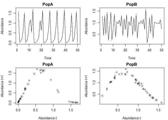
Here is how you might set up a hierarchical time-delay embedding model. In this example, Abundance is the response variable (y). We will use an embedding dimension (E) of 3 and time delay (tau) of 1. Population indicates which population the data are from, so it is included under pop. Since the data are on somewhat different scales and don’t necessarily represent the same ‘units’, we will use local (within population) data scaling, as opposed to global. Just for fun, we will also request leave-one-out predictions.
tlogtest=fitGP(data = thetalog2pop, y = "Abundance", pop = "Population", E=3, tau=1,
               scaling = "local", predictmethod = "loo")
summary(tlogtest)
#> Number of predictors: 3
#> Length scale parameters:
#>        predictor posteriormode
#> phi1 Abundance_1        0.5317
#> phi2 Abundance_2        0.0000
#> phi3 Abundance_3        0.0000
#> Process variance (ve): 0.01222333
#> Pointwise prior variance (sigma2): 2.527349
#> Number of populations: 2
#> Dynamic correlation (rho): 0.327254
#> In-sample R-squared: 0.9933975
#> In-sample R-squared by population:
#>             R2
#> PopA 0.9970811
#> PopB 0.9815187
#> Out-of-sample R-squared: 0.991238
#> Out-of-sample R-squared by population:
#>             R2
#> PopA 0.9961280
#> PopB 0.9754702
From the summary, we can see that ARD has (unsurprisingly) deemed lags 2 and 3 to be unimportant (length scales are 0), so E=1 is probably sufficient. The dynamic correlation (rho) tells us the degree to which the dynamics are correlated (they are are rather dissimilar in this case). Since the simulated data don’t contain that much noise, the R-squared values are quite high. For more information on choosing embedding parameters, see this vignette. For more information on hierarchical modeling and the dynamic correlation, see this other vignette.
Plot observed and predicted values
The observed and predicted values can be found under model$insampresults or model$outsampresults.
We can make a quick plot of the observed and predicted values using plot. Standard error bands are included in the time series plots, although they’re a little hard to see in this example.
plot(tlogtest)
#> Plotting out of sample results.
To get the in-sample predictions:
plot(tlogtest, plotinsamp = T)
#> Plotting in sample results.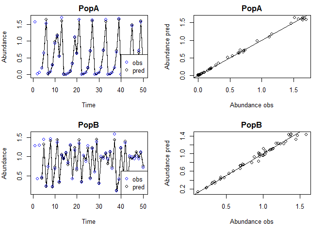
If you prefer ggplot:
library(ggplot2)
ggplot(tlogtest$insampresults,aes(x=timestep,y=predmean)) +
  facet_wrap(pop~., scales = "free") +
  geom_line() + geom_ribbon(aes(ymin=predmean-predfsd,ymax=predmean+predfsd), alpha=0.4) +
  geom_point(aes(y=obs)) +
  theme_bw()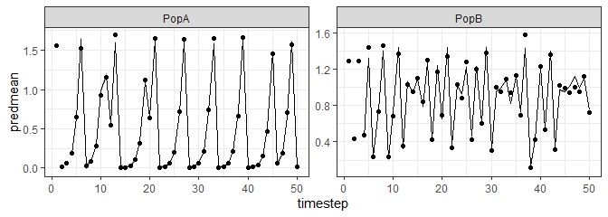
Plot conditional responses
The function getconditionals will compute and plot conditional responses to each input variable (other input varibles set to their mean value). From this we can also clearly see that lags 2 and 3 have no impact, and we can see how the lag 1 dynamics of the 2 populations differ.
con=getconditionals(tlogtest)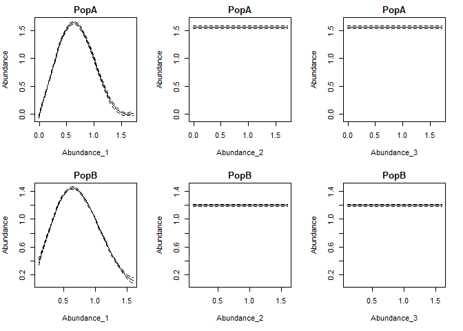
If you prefer ggplot:
#have to convert conditionals output to long format
#there may be a more concise way to do this
library(tidyr)
npreds=length(grep("_yMean",colnames(con)))
conlong1=gather(con[,1:(npreds+1)],x,xValue,2:(npreds+1))
conlong2=gather(con[,c(1,(npreds+2):(2*npreds+1))],ym,yMean,2:(npreds+1))
conlong3=gather(con[,c(1,(2*npreds+2):(3*npreds+1))],ys,ySD,2:(npreds+1))
conlong=cbind.data.frame(conlong1,yMean=conlong2$yMean,ySD=conlong3$ySD)
ggplot(conlong,aes(x=xValue,y=yMean)) +
  facet_grid(pop~x, scales = "free") +
  geom_line() + geom_ribbon(aes(ymin=yMean-ySD,ymax=yMean+ySD), alpha=0.4) +
  theme_bw()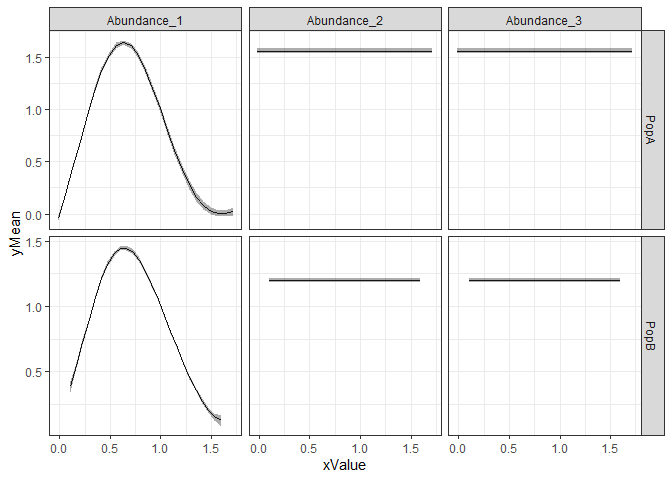
Plot inverse length scales
The model hyperparameters are located under model$pars. If you have predictors, the first values of pars will be the length scales. Note that if you use E and tau, the names of the predictors in the input data frame will be stored under model$inputs$x_names, and the names of the lagged predictors corresponding to the inverse length scales will be stored under model$inputs$x_names2.
predvars=tlogtest$inputs$x_names2
npreds=length(predvars)
lscales=tlogtest$pars[1:npreds]
par(mar=c(4,4,1,1))
plot(factor(predvars),lscales,xlab="Predictor",ylab="Inverse length scale")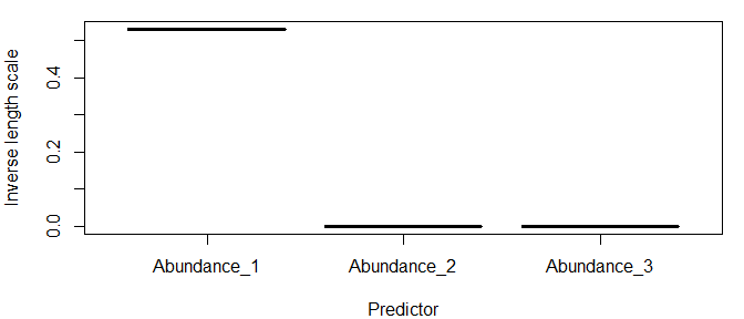
Other types of predictions
We can use the predict function to get various types of predictions from a fitted model. Leave-one-out, predictmethod = "loo" is one option (above, we got these predictions at the same time we fit the model, but this is not necessary). The following obtains sequential (leave-future-out) predictions using the training data. Note that for predictmethod = "loo" and predictmethod = "sequential", the training data are iteratively omitted for the predictions, but the hyperparameter values used are those obtained using all of the training data (the model is not refit).
#sequential predictions (they should improve over time)
seqpred=predict(tlogtest,predictmethod = "sequential")
plot(seqpred)
#> Plotting out of sample results.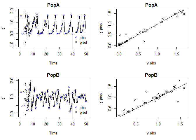
You could, alternatively, supply new data for which to make predictions. In that case, you would supply a new data frame (newdata). In our example, this data frame which should contain columns Abundance and Population.
A common approach when fitting these models is to split the available data into a training and test dataset. For instance, say we wanted a single-population model for PopA with 2 time lags, and we wanted to use the first 40 data points as training data, and the last 10 points as test data. For that we could do the following.
pAtrain=pA[1:40,]
pAtest=pA[41:50,]
tlogtest2=fitGP(data = pAtrain, y = "Abundance", E=2, tau=1, time = "Time", newdata = pAtest)
plot(tlogtest2)
#> Plotting out of sample results.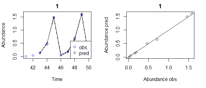
If you don’t want the first E*tau points getting excluded from your test data, generate the lags beforehand, then split the data (don’t use E and tau options in fitGP). See Specifying training data (option 1).
pAlags=makelags(pA, y = "Abundance", E=2, tau=1)
pAdata=cbind(pA,pAlags)
pAtrain=pAdata[1:40,]
pAtest=pAdata[41:50,]
tlogtest3=fitGP(data = pAtrain, y = "Abundance", x=colnames(pAlags), time = "Time", newdata = pAtest)
plot(tlogtest3)
#> Plotting out of sample results.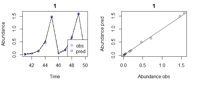
Note that this is equivalent to:
Simulating forecasts
The function predict_seq also generates predictions for a data frame newdata, but sequentially adds each new observation to the training data and refits the model. This simulates a real-time forecasting application. This prediction method is similar to predictmethod="sequential" (leave-future-out), but in this case, the future time points are not included in the training data used to obtain the hyperparameters. It is also similar to the train/test split using newdata, but in this case, the training data and model hyperparameters are sequentially updated with each timestep. Use of this method requires the use of data with pre-generated lags (see Specifying training data, option A1), that a time column is specified, that newdata has exactly the same columns as data, and that newdata has observed values.
tlogtest3_update=predict_seq(tlogtest3, newdata=pAtest)

summary(tlogtest3)
#> Number of predictors: 2
#> Length scale parameters:
#>        predictor posteriormode
#> phi1 Abundance_1       0.62609
#> phi2 Abundance_2       0.00000
#> Process variance (ve): 0.003394526
#> Pointwise prior variance (sigma2): 2.331728
#> Number of populations: 1
#> In-sample R-squared: 0.9971411

summary(tlogtest3_update)
#> Number of predictors: 2
#> Length scale parameters:
#>        predictor posteriormode
#> phi1 Abundance_1       0.59103
#> phi2 Abundance_2       0.00000
#> Process variance (ve): 0.003158423
#> Pointwise prior variance (sigma2): 2.389629
#> Number of populations: 1
#> In-sample R-squared: 0.9972318
#> Out-of-sample R-squared: 0.9973224

plot(tlogtest3_update)
#> Plotting out of sample results.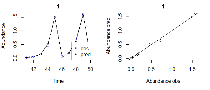
Making forecasts
You can also use predict to generate predictions beyond the end of the training data. You can construct a forecast matrix extending beyond the last timepoint using makelags and setting forecast=T. This can be supplied this as newdata. To use this method, you have to generate the lags beforehand for both the training data and the forecast (use makelags for both, and the settings in makelags should match, other than forecast, see Specifying training data option 1). It is a good idea to include the time argument when doing this.
lags1=makelags(thetalog2pop,y=c("Abundance"),pop="Population",time="Time",E=3,tau=1)
fore1=makelags(thetalog2pop,y=c("Abundance"),pop="Population",time="Time",E=3,tau=1,forecast = T)
data1=cbind(thetalog2pop, lags1)

tail(data1)
#>     Time Population Abundance Abundance_1 Abundance_2 Abundance_3
#> 95    45       PopB 0.9940592   1.0237266   0.3177380   1.3631716
#> 96    46       PopB 0.9388969   0.9940592   1.0237266   0.3177380
#> 97    47       PopB 1.0032245   0.9388969   0.9940592   1.0237266
#> 98    48       PopB 0.9477896   1.0032245   0.9388969   0.9940592
#> 99    49       PopB 1.1221056   0.9477896   1.0032245   0.9388969
#> 100   50       PopB 0.7238974   1.1221056   0.9477896   1.0032245

fore1
#>   Time Population Abundance_1 Abundance_2 Abundance_3
#> 1   51       PopA  0.01543102    1.574257   0.7120728
#> 2   51       PopB  0.72389740    1.122106   0.9477896

tlogfore=fitGP(data = data1, y = "Abundance", x=c("Abundance_1","Abundance_2","Abundance_3"),
               pop = "Population", time = "Time", scaling = "local", newdata = fore1)

ggplot(tlogfore$insampresults,aes(x=timestep,y=predmean)) +
  facet_wrap(pop~., scales = "free") +
  geom_line() + geom_ribbon(aes(ymin=predmean-predsd,ymax=predmean+predsd), alpha=0.4) +
  geom_point(aes(y=obs)) +
  geom_point(data=tlogfore$outsampresults, aes(y=predmean), color="red") +
  geom_errorbar(data=tlogfore$outsampresults,
                aes(ymin=predmean-predsd,ymax=predmean+predsd),color="red") +
  theme_bw()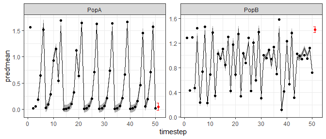
Making iterated forecasts
The predict_iter function can be used to obtain iterated predictions from fitGP models with lag predictors. This method also requires pre-generated lags and the use of newdata (see Specifying training data option 1). The time argument is required.
Starting with the first row of newdata, the predicted y variable is inserted as the first lag for the next timestep, the other lags are shifted right by 1, and a new prediction is made. This continues for as many rows as are in newdata. Thus, this procedure assumes that all lags are present, evenly spaced, and in order (first lag is the first column). Time steps are assumed to be evenly spaced. The units of y and its lags are assumed to be the same.
Unless otherwise specified, all values of x are assumed to be time lags of y. If this is not the case (the model contains a mixture of lags and covariates), you must specify which columns are the time lags (argument xlags in predict_iter). The exception is for “fisheries models” (fitGP_fish), where the lags and covariates are already separately specified.
As with other prediction methods, newdata should contain all values of x, as well as time. Only the first row of lags in newdata (for each population) needs to be completely filled in. Subsequent time points can be NA or filled in - they will be overwritten with the predictions as the model iterates. The values of time and must be filled in. If the model has covariates, values for the covariates need to be supplied for all timepoints in newdata. If there are multiple populations, newdata should contain pop and there should be duplicated timesteps for each population.
As expected for a chaotic system, the iterated predictions from the simulated 2 population theta logistic model become very poor after a few timesteps.
xdata=makelags(data = thetalog2pop, y="Abundance", pop="Population", time = "Time", E=3, tau=1, append=T)
xdatatrain=subset(xdata, Time<=40)
#get iterated predictions for the last 10 timesteps
xdatafore=subset(xdata, Time>40)

tlog=fitGP(data = xdatatrain, y = "Abundance", x=c("Abundance_1","Abundance_2","Abundance_3"),
           pop = "Population", time = "Time", scaling = "local")
predtest=predict_iter(tlog, newdata = xdatafore)

plot(predtest)
#> Plotting out of sample results.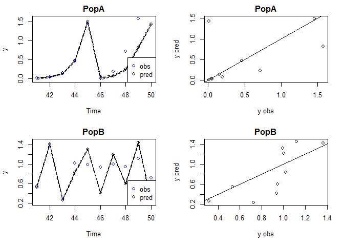
If you want to iterate forecasts beyond the end of the time series, here is how you might set that up. Note that because there are no observed values, we can’t evaluate fit or make plots of observed vs. predicted.
xdata=makelags(data = thetalog2pop, y="Abundance", pop="Population", time="Time", E=3, tau=1, append=T)
#use forecast feature to get first rows
xdatafore=makelags(data = thetalog2pop, y="Abundance", pop="Population", time="Time", E=3, tau=1, forecast=T)
#create remaining timepoints for each population
xdatafore2=expand.grid(Time=52:65, Population=unique(thetalog2pop$Population))
#create empty matrix for future values
xdatafore3=matrix(NA, nrow=nrow(xdatafore2), ncol=3,
                  dimnames=list(NULL,c("Abundance_1","Abundance_2","Abundance_3")))
#combine everything
xdatafore=rbind(xdatafore,cbind(xdatafore2,xdatafore3))

head(xdatafore)
#>   Time Population Abundance_1 Abundance_2 Abundance_3
#> 1   51       PopA  0.01543102    1.574257   0.7120728
#> 2   51       PopB  0.72389740    1.122106   0.9477896
#> 3   52       PopA          NA          NA          NA
#> 4   53       PopA          NA          NA          NA
#> 5   54       PopA          NA          NA          NA
#> 6   55       PopA          NA          NA          NA

tlog2=fitGP(data = xdata, y = "Abundance", x=c("Abundance_1","Abundance_2","Abundance_3"),
           pop = "Population", time = "Time", scaling = "local")
predtest2=predict_iter(tlog2, newdata = xdatafore)
#plot(predtest2)
head(predtest2$outsampresults)
#>   timestep  pop   predmean    predfsd     predsd
#> 1       51 PopA 0.04932054 0.01647408 0.06829043
#> 2       51 PopB 1.41625389 0.01679414 0.04612410
#> 3       52 PopA 0.15774996 0.01367564 0.06766986
#> 4       52 PopB 0.26582495 0.01688767 0.04615824
#> 5       53 PopA 0.53367538 0.01829694 0.06875293
#> 6       53 PopB 0.83186406 0.01782242 0.04650837
Specifying training data
There are several ways that the training data for a model can be specified.
A. supply data frame data, plus column names or indices for y and x.
B. supply a vector for y and a vector or matrix for x.
For each of the above 2 options, there are 3 options for specifying the predictors.
- supplying
yandx(omittingEandtau) will use the columns ofxas predictors. This allows for the most customization.
- supplying
y,E, andtau(omittingx) will useElags ofy(with spacingtau) as predictors. This is equivalent to option 3 withx=y.
- supplying
y,x,E, andtauwill useElags of each column ofx(with spacingtau) as predictors. Do not use this option ifxalready contains lags, in that case use option 1.
The above examples use methods A2 and A1.
Option 1 allows for the most customization of response and predictor variables, including use of mixed embeddings, and use of different variables for the response and predictors. Options 2 and 3 exist for convenience, but for the most control over the model and to use the more elaborate features in this package, it is best to use option 1: use makelags to generate any lags beforehand and pass appropriate columns to fitGP, rather than rely on fitGP to generate lags internally. Option A will make more sense if your data are already in a data frame, option B may make more sense if you are doing simulations and just have a bunch of vectors and matrices.
The pop argument is optional in all of the above cases. Beware that if omitted, a single population is assumed.
set.seed(10)
thetalog2pop$othervar=rnorm(nrow(thetalog2pop))
yvec=thetalog2pop$Abundance
popvec=thetalog2pop$Population
#function 'makelags' can be used to generate a lag matrix
#be sure to include 'pop' if data contain multiple pops to prevent crossover
xmat=makelags(y=thetalog2pop[,c("Abundance","othervar")],pop=popvec,E=2,tau=1)
thetalog2pop2=cbind(thetalog2pop,xmat)

#Method A1
ma1=fitGP(data=thetalog2pop2,y="Abundance",x=c("Abundance_1","othervar"),
         pop="Population",scaling="local")

#Method B1
#like A1, but your data aren't in a data frame
mb1=fitGP(y=yvec,x=xmat,pop=popvec,scaling="local")

#Method B2
#like A2, but your data aren't in a data frame
mb2=fitGP(y=yvec,pop=popvec,E=2,tau=1,scaling="local")

#Method A3
#generate lags of multiple predictors internally
ma3=fitGP(data=thetalog2pop2,y="Abundance",x=c("Abundance","othervar"),
         pop="Population",E=2,tau=1,scaling="local")


summary(ma1)
#> Number of predictors: 2
#> Length scale parameters:
#>        predictor posteriormode
#> phi1 Abundance_1       0.52284
#> phi2    othervar       0.00030
#> Process variance (ve): 0.01031377
#> Pointwise prior variance (sigma2): 2.51944
#> Number of populations: 2
#> Dynamic correlation (rho): 0.2924004
#> In-sample R-squared: 0.9945158
#> In-sample R-squared by population:
#>             R2
#> PopA 0.9971671
#> PopB 0.9855357

summary(mb1)
#> Number of predictors: 4
#> Length scale parameters:
#>        predictor posteriormode
#> phi1 Abundance_1       0.50864
#> phi2 Abundance_2       0.00000
#> phi3  othervar_1       0.00028
#> phi4  othervar_2       0.00000
#> Process variance (ve): 0.01026616
#> Pointwise prior variance (sigma2): 2.688766
#> Number of populations: 2
#> Dynamic correlation (rho): 0.2901182
#> In-sample R-squared: 0.9945261
#> In-sample R-squared by population:
#>             R2
#> PopA 0.9971058
#> PopB 0.9856039

summary(mb2)
#> Number of predictors: 2
#> Length scale parameters:
#>      posteriormode
#> phi1       0.53026
#> phi2       0.00000
#> Process variance (ve): 0.01205454
#> Pointwise prior variance (sigma2): 2.540002
#> Number of populations: 2
#> Dynamic correlation (rho): 0.3250384
#> In-sample R-squared: 0.9935199
#> In-sample R-squared by population:
#>             R2
#> PopA 0.9971163
#> PopB 0.9817038

summary(ma3)
#> Number of predictors: 4
#> Length scale parameters:
#>        predictor posteriormode
#> phi1 Abundance_1       0.50864
#> phi2 Abundance_2       0.00000
#> phi3  othervar_1       0.00028
#> phi4  othervar_2       0.00000
#> Process variance (ve): 0.01026616
#> Pointwise prior variance (sigma2): 2.688766
#> Number of populations: 2
#> Dynamic correlation (rho): 0.2901182
#> In-sample R-squared: 0.9945261
#> In-sample R-squared by population:
#>             R2
#> PopA 0.9971058
#> PopB 0.9856039
Gradient of the GP
The partial derivatives of the fitted GP function at each time point with respect to each input can be obtained from the predict function, setting returnGPgrad = T. They will be under model$GPgrad. The gradient will be computed for each out-of-sample prediction point requested (using methods "loo", "lto", or newdata). If you want the in-sample gradient, pass the original (training) data as back in as newdata.
grad1=predict(tlogtest, predictmethod = "loo", returnGPgrad = T)
gradplot=cbind(grad1$outsampresults,grad1$GPgrad, lags1)

par(mfrow=c(2,2),mar=c(4,4,2,1))
plot(predmean~Abundance_1, data=subset(gradplot, pop=="PopA"), main="PopA")
plot(predmean~Abundance_1, data=subset(gradplot, pop=="PopB"), main="PopB")
plot(d_Abundance_1~Abundance_1, data=subset(gradplot, pop=="PopA"), main="PopA"); abline(h=0)
plot(d_Abundance_1~Abundance_1, data=subset(gradplot, pop=="PopB"), main="PopB"); abline(h=0)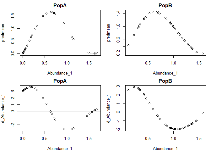
More examples:
grad2=predict(tlogtest3, newdata = pAtest, returnGPgrad = T)
grad2$GPgrad

#it can also be done at the same time as model fitting
tlogtest3=fitGP(data = pAtrain, y = "Abundance", x=colnames(pAlags), time = "Time",
                newdata = pAtest, returnGPgrad = T)

#in sample
grad3=predict(tlogtest3, newdata = pAtrain, returnGPgrad = T)
Extensions
See this vignette for more detail about the variable timestep method (VS-EDM) for missing data.
See this vignette for more detail on an alternative parameterization of the GP model, fitGP_fish, designed for use in fisheries applications.
References
Munch, S. B., Poynor, V., and Arriaza, J. L. 2017. Circumventing structural uncertainty: a Bayesian perspective on nonlinear forecasting for ecology. Ecological Complexity, 32:134.
Johnson, B., and Munch, S. B. 2022. An empirical dynamic modeling framework for missing or irregular samples. Ecological Modelling, 468:109948.
Any advice on improving this package is appreciated.
Disclaimer
“This repository is a scientific product and is not official communication of the National Oceanic and Atmospheric Administration, or the United States Department of Commerce. All NOAA GitHub project code is provided on an ‘as is’ basis and the user assumes responsibility for its use. Any claims against the Department of Commerce or Department of Commerce bureaus stemming from the use of this GitHub project will be governed by all applicable Federal law. Any reference to specific commercial products, processes, or services by service mark, trademark, manufacturer, or otherwise, does not constitute or imply their endorsement, recommendation or favoring by the Department of Commerce. The Department of Commerce seal and logo, or the seal and logo of a DOC bureau, shall not be used in any manner to imply endorsement of any commercial product or activity by DOC or the United States Government.”