Choosing Embedding Parameters • GPEDM

library(GPEDM)
library(ggplot2)

Introduction

One of the most common questions we get is how to choose the embedding dimension $E$ and time delay $\tau$ for a given time series. There is, unfortunately, no one correct way to do this. We detail below some general guidelines and different approaches that can be used to select these values.

The maximum embedding dimension that can be estimated for a time series of length $T$ is approximately $\sqrt{T}$ (Cheng and Tong 1992), so the largest $E$ considered should not exceed this too greatly. The actual attractor dimension of the system may be higher, but the dimension you’re going to be able to resolve will be limited by time series length. You also may have valid reasons to limit the largest $E$ considered to something less than $\sqrt{T}$ . Note that in multivariate models (e.g. those with covariates) $E$ is the total number of predictors including lags, covariates, and lags of covariates. The total number of predictors should not exceed $\sqrt{T}$ , meaning you may need to use fewer lags if you add covariates to the model. For example, $\{x_{t-1},x_{t-2},x_{t-3}\}$ , $\{x_{t-1},x_{t-2},y_{t-1}\}$ , and $\{x_{t-1},y_{t-1},z_{t-1}\}$ are all 3-dimensional embeddings ( $E=3$ ).

In terms of selecting $\tau$ , fixing it to 1 can be a completely justifiable approach, particularly if your sampling interval is coarse relative to the dynamics of the system. However, if the sampling interval is fine, or the timescale of dynamics uncertain, you might wish to explore other values of $\tau$ . The generation time of the species under study (if longer than the sampling interval) can sometimes provide a good ballpark estimate for $\tau$ . The first zero crossing of the autocorrelation function is another method proposed for identifying $\tau$ , although this is most suitable for continuous time systems, and may not work as well for discrete time systems.

If you have multiple series, then the maximum $E$ can be based on the total number of time points across all series, provided that the product $E\tau$ is less than the length of the shortest individual time series. For example, if you have 100 replicate series that are each only 5 time points long, you may have 500 data points, but you can’t use $E$ more than 5 (or $E\tau>5$ ) because for no point do you know $y_{t-6}$ , and you will end up with zero usable delay vectors.

Also keep in mind that $E\tau$ data points will always be lost from the beginning of the time series (or each time series), as well as after every missing data point (if you are keeping them in and skipping them). In the absence of a long, continuous time series, you might want to set some threshold for the amount of data lost when constructing lags, so that you end up with a sufficient number of valid delay vectors. For instance, when evaluating possible $E$ and $\tau$ values for S-map EDM, Rogers et al. (2022) required both $E\leq \sqrt{T}$ and $E\tau\leq 0.2T$ (i.e. you cannot remove more than 20% of the data points). So, larger values of $E$ could be tested when $\tau$ was small.

Once you have identified a space of reasonable $E$ and $\tau$ combinations to consider, there are a variety of methods you can use to select them (either independently or jointly). The false nearest neighbors approach is one method for identifying $E$ that can be successful, but since it requires defining a threshold at which point neighbors are or are not considered ‘false’, it can be difficult to apply consistently across various time series. The Grassberger-Procacia algorithm is another, but it tends to be sensitive to noise and sample size. Both also assume a fixed $\tau$ . More commonly, $E$ and $\tau$ are selected jointly using some metric of out-of-sample model performance and a grid search. Note that because $E$ and $\tau$ are discrete quantities, there is no ‘gradient’ that can be derived to find a best value using likelihood based optimizers; they have to be found by trial and error.

GP-EDM includes automatic relevance determination (ARD), which enables some additional strategies for choosing $E$ and $\tau$ beyond the grid search. ARD involves placing priors on the inverse length scale parameters with a mode of 0 (akin to a wiggliness penalty) that effectively eliminates uninformative lags, so can be used (in theory) to automatically identify $E$ and choose the relevant time lags ( $\tau$ values).

We present a few possible methods below, which are based on model performance. Note that performance must be evaluated out-of-sample, e.g. using leave-one-out cross validation, a training/test split, or some other method (which method to use will depend on how much data you have). In-sample performance will always increase as $E$ increases, but out-of-sample performance will cease to improve substantially once the optimal $E$ is reached.

Because real data are rarely as cooperative as models, we present both a model example (noise-free, 3 species Hastings-Powell model) and a real data example (shortfin squid mean catch-per-unit-effort from a bottom trawl survey in the Gulf of Maine) for each method.

1. Grid search method

Evaluate all possible models and select the best performing. This is the most computationally intensive, but also the most thorough, and the only option if the hyperparameters that cannot be optimized numerically. For instance, Rogers et al. (2022) found that the best approach in S-map EDM was to evaluate all possible combinations of $E$ , $\tau$ , and the S-map local weighting parameter $\theta$ and choose the one with the highest out-of-sample $R^2$ . (It is worth pointing out that if you do a giant search like this with ‘out-of-sample’ $R^2$ , you probably want to also do an ‘out-of-out-of-sample’ evaluation of the end product, if sufficient data exist. For example, have a training, test, and validation dataset.)

Performance may or may not reach a maximum as you increase $E$ ; it may simply plateau, where beyond a certain $E$ , models are effectively equivalent and there is no ‘appreciable’ gain in performance. In this case, you will probably want to choose the simplest (lowest $E$ ) model of the plateau, rather than model at the actual maximum, if that maximum performance differs little from the performance of the simpler model. This could be made more rigorous by including a penalty for the degrees of freedom in the performance metric.

When evaluating a large number of possible models, you can run into identifiability issues, in that multiple models can have identical or near identical fits. For example, a periodic time series with a period of 4 can be perfectly described with $E$ / $\tau$ combinations of 2/1, 4/1, 2/2, 1/4, 1/8, etc. It can be useful to establish criteria for determining which models are effectively equivalent (e.g. they differ by less than 0.01 in $R^2$ ), and how equivalent models should be ranked (e.g. prioritize simpler, more linear models). For example, Rogers et al. (2022) selected the one with the lowest $\tau$ , $\theta$ , and $E$ (in that order). This is particularly problematic in simulated data with little to no noise, where many different models can have high fit statistics, but can happen with real data as well, where there is not a clear ‘winner’ among the candidate models.

Since the inverse length scales in GP-EDM are optimized using gradient descent, this leaves just the values of $E$ and $\tau$ that need to be determined. However, running an entire grid search with GP-EDM is probably unnecessary because of ARD, and you could instead use one of the other methods.

Hastings Powell model

Since we have plenty of simulated data, we’ll split the time series into a training and testing set, each of 200 points. To ensure that the out-of-sample $R^2$ is evaluated over the same test set regardless of $E$ and $\tau$ (the first $E\tau$ points of the test dataset are not eliminated), we generate the lags beforehand (see the last example in this section of the readme). With 200 points, we could consider $E$ up to 14, but since we know that is far higher than necessary for this model system, we’ll set max $E$ to 8 to save some time.

We find that $E=2$ and $\tau=1$ are sufficient here. This is a continuous time model with an integration step size of 1, so it is also not surprising that higher $\tau$ values work well as long as $E$ is at least 2.

#we'll just consider the X variable
qplot(y=X, x=Time, data=HastPow3sp, geom = "line")
#> Warning: `qplot()` was deprecated in ggplot2 3.4.0.
#> This warning is displayed once every 8 hours.
#> Call `lifecycle::last_lifecycle_warnings()` to see where this warning was
#> generated.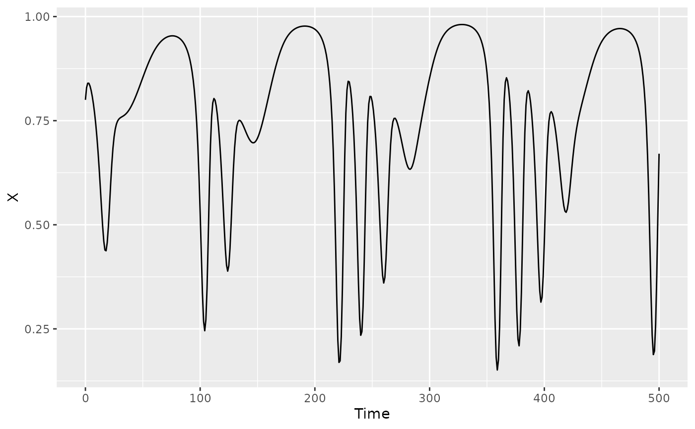


#create grid of E and tau to consider
Emax=8
taumax=3
Etaugrid=expand.grid(E=1:Emax,tau=1:taumax)
Etaugrid$R2=NA

#generate all lags
HPlags=makelags(HastPow3sp,"X",E=Emax*taumax, tau=1, append=T)

#split training and test
HP_train=HPlags[1:200,]
HP_test=HPlags[201:400,]

#loop through the grid
for(i in 1:nrow(Etaugrid)) {
  #fit model with ith combo of E and tau
  demo=fitGP(data=HP_train, 
             y="X",
             x=paste0("X_",Etaugrid$tau[i]*(1:Etaugrid$E[i])), 
             time="Time", 
             newdata = HP_test)
  #store out of sample R2
  Etaugrid$R2[i]=demo$outsampfitstats["R2"]
}

ggplot(Etaugrid, aes(x=E, y=tau, fill=R2)) +
  geom_tile() + theme_classic() +
  scale_y_continuous(expand = c(0, 0), breaks = 1:taumax) +
  scale_x_continuous(expand = c(0, 0), breaks = 1:Emax) +
  scale_fill_gradient2() +
  theme(panel.background = element_rect(fill="gray"), 
        panel.border = element_rect(color="black", fill="transparent"))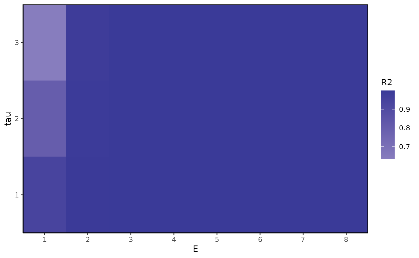


Etaugrid$R2round=round(Etaugrid$R2,2)
#if not aleady in order
#Etaugrid=Etaugrid[order(Etaugrid$tau,Etaugrid$E),] 
(bestE=Etaugrid$E[which.max(Etaugrid$R2round)])
#> [1] 2
(besttau=Etaugrid$tau[which.max(Etaugrid$R2round)])
#> [1] 1

demo=fitGP(data=HP_train, y="X",
           x=paste0("X_",besttau*(1:bestE)),
           time="Time", newdata = HP_test)
summary(demo)
#> Number of predictors: 2 
#> Length scale parameters:
#>      predictor posteriormode
#> phi1       X_1       0.21716
#> phi2       X_2       0.33140
#> Process variance (ve): 0.0001761443
#> Pointwise prior variance (sigma2): 4.365049
#> Number of populations: 1
#> In-sample R-squared: 0.9998473 
#> Out-of-sample R-squared: 0.9979118
plot(demo)
#> Plotting out of sample results.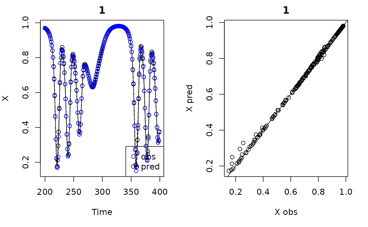

Squid data

This is 44 year annual time series, thus the max $E$ should be about 6 or 7. The squid species being sampled has an annual life history, so tau=1 would make the most biological sense. Just for demonstration purposes, we set the max $\tau$ to 3. To provide a more complex example in which the predictor and response variables are different, we will model growth rate as a function of log abundance (we will need to generate the lags beforehand, option 1 in Specifying training data). Because the time series is relatively short, we will use leave-one-out to evaluate performance.

We find that $\tau=1$ is clearly the best, and $E=6$ produces the best performance, although only minorly over $E=4$ (they differ in $R^2$ by only 0.0102). You would be justified in selecting either $E=4$ or $E=6$ , perhaps going for the smaller one if you were interested in parsimony.

#we'll just consider one population for this example
data(trawl)
squid=subset(trawl,REGION=="GME")
qplot(y=shortfin_squid, x=YEAR, data=squid, geom = "line")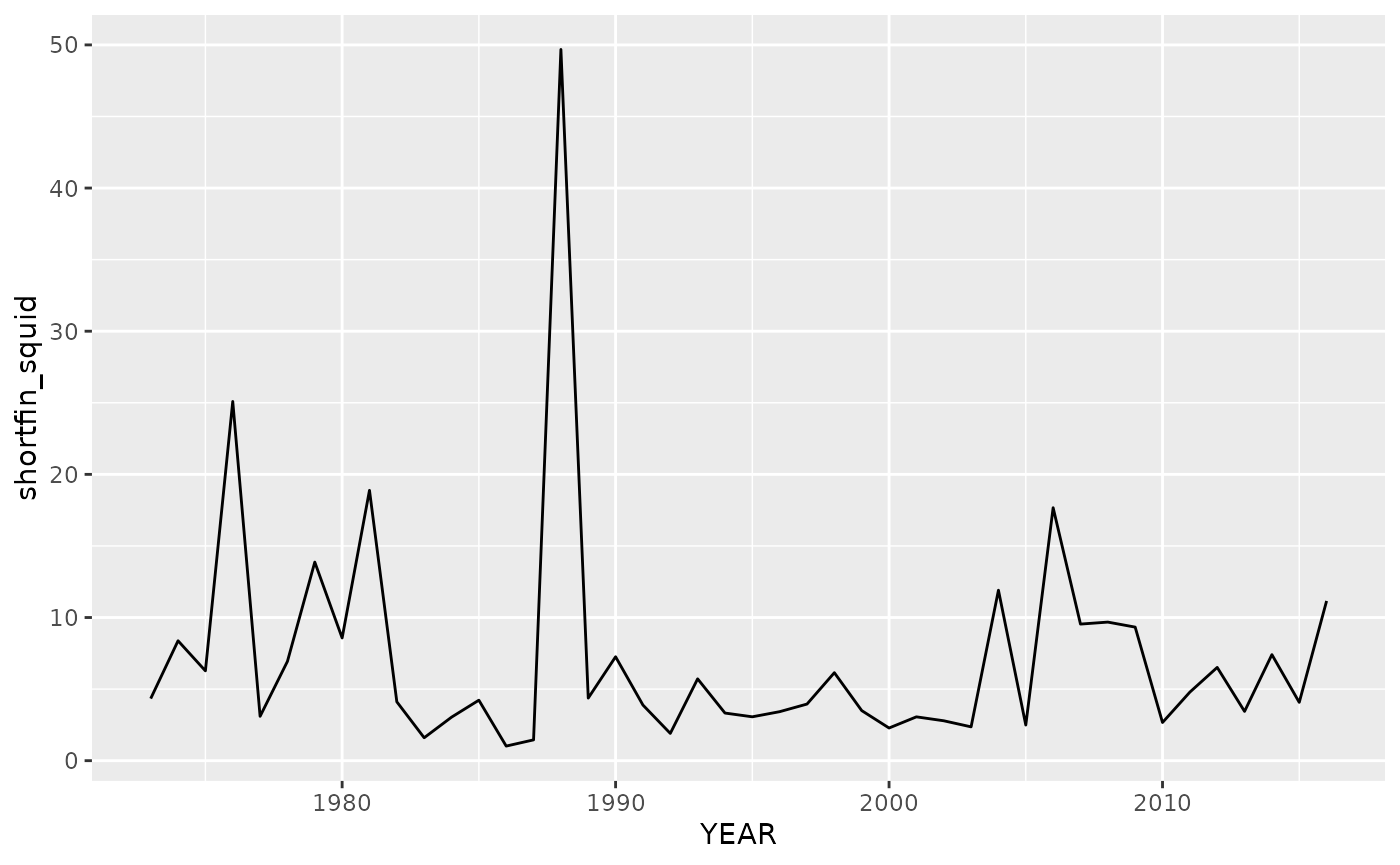


#growth rate and log abundance
squid$squidlog=log(squid$shortfin_squid)
squid$squidgr=c(NA,(diff(squid$squidlog)))
#time series length
serlen=nrow(squid)

#create grid of E and tau to consider
Emax=6
taumax=3
Etaugrid=expand.grid(E=1:Emax,tau=1:taumax)
#remove E and tau combinations that lose too much data (other critera could be used)
Etaugrid=subset(Etaugrid, Etaugrid$E^2<=serlen & Etaugrid$E*Etaugrid$tau/serlen<=0.2)
Etaugrid$R2=NA

#generate all lags
squidlags=makelags(squid,"squidlog",E=Emax*taumax, tau=1, append=T)

#loop through the grid
for(i in 1:nrow(Etaugrid)) {
  #fit model with ith combo of E and tau
  demo=fitGP(data=squidlags, 
             y="squidgr",
             x=paste0("squidlog_",Etaugrid$tau[i]*(1:Etaugrid$E[i])), 
             time="YEAR", 
             predictmethod = "loo")
  #store out of sample R2
  Etaugrid$R2[i]=demo$outsampfitstats["R2"]
}

ggplot(Etaugrid, aes(x=E, y=tau, fill=R2)) +
  geom_tile() + theme_classic() +
  scale_y_continuous(expand = c(0, 0), breaks = 1:taumax) +
  scale_x_continuous(expand = c(0, 0), breaks = 1:Emax) +
  scale_fill_gradient2() +
  theme(panel.background = element_rect(fill="gray"), 
        panel.border = element_rect(color="black", fill="transparent"))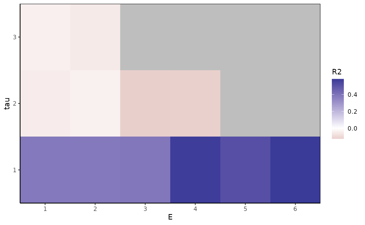


Etaugrid$R2round=round(Etaugrid$R2,2)
#if not aleady in order
#Etaugrid=Etaugrid[order(Etaugrid$tau,Etaugrid$E),] 
(bestE=Etaugrid$E[which.max(Etaugrid$R2round)])
#> [1] 6
(besttau=Etaugrid$tau[which.max(Etaugrid$R2round)])
#> [1] 1

demo=fitGP(data=squidlags, y="squidgr", 
           x=paste0("squidlog_",besttau*(1:bestE)),
           time="YEAR", 
           predictmethod = "loo")
summary(demo)
#> Number of predictors: 6 
#> Length scale parameters:
#>       predictor posteriormode
#> phi1 squidlog_1       0.04734
#> phi2 squidlog_2       0.24373
#> phi3 squidlog_3       0.06569
#> phi4 squidlog_4       0.00746
#> phi5 squidlog_5       0.02067
#> phi6 squidlog_6       0.00130
#> Process variance (ve): 0.203274
#> Pointwise prior variance (sigma2): 2.647853
#> Number of populations: 1
#> In-sample R-squared: 0.8892768 
#> Out-of-sample R-squared: 0.5833364
plot(demo)
#> Plotting out of sample results.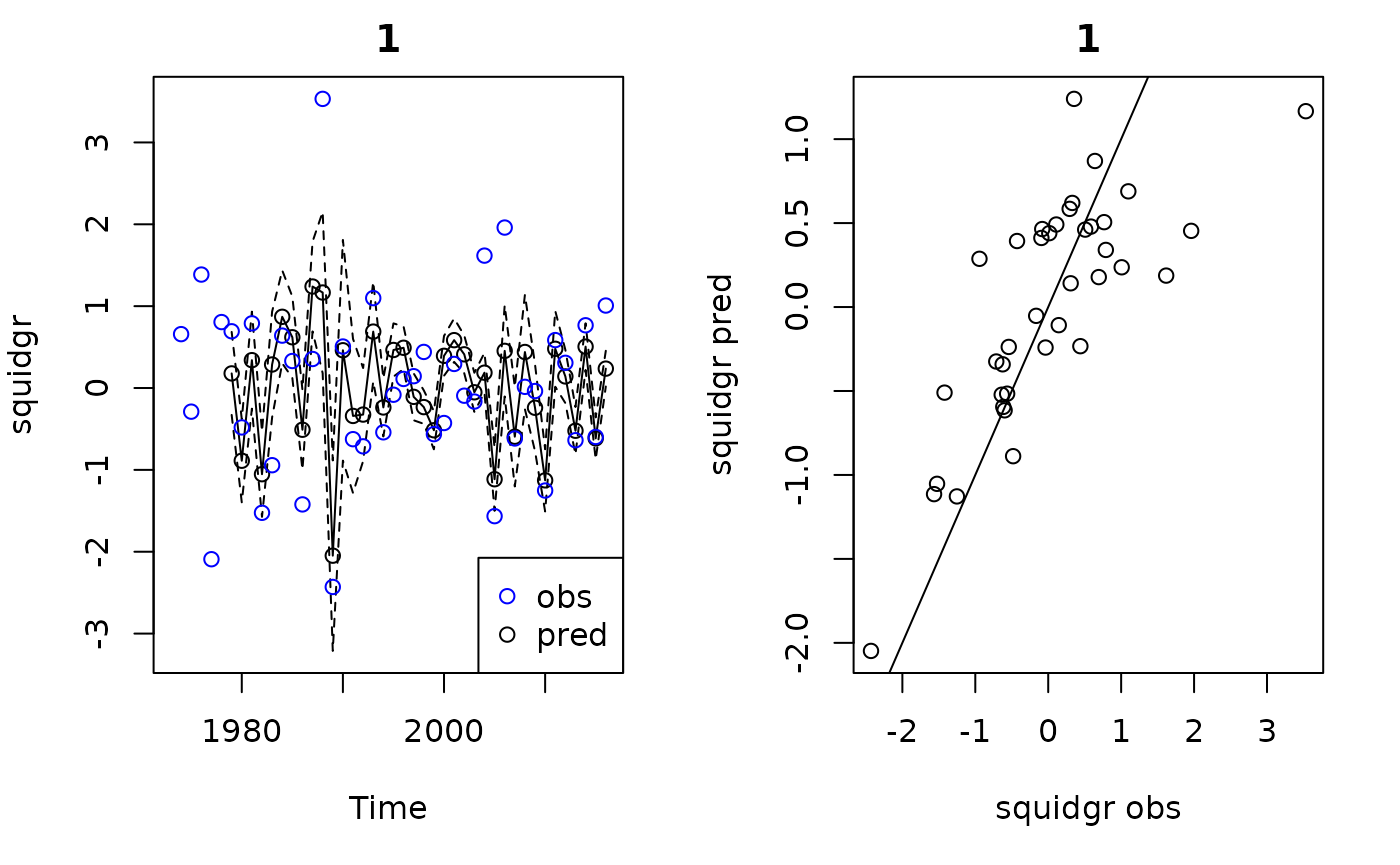

This grid search method of selecting models, while thorough, can be very time consuming. There are some potentially more efficient ways to arrive at the same answer, described below.

2. Increase E method

Increase $E$ until performance no longer increases substantially (fixing $\tau$ to 1 or some other reasonable minimum value). ARD will drop lags that are uninformative, allowing for a larger ‘realized’ $\tau$ , as well as unequal lag spacing. You might notice that the set of relevant lags changes as $E$ increases (e.g. lag 2 is important when $E=2$ , but not when $E=4$ ). This behavior is normal and occurs because lags sometimes provide redundant information, and thus the model will identify different lags as relevant depending on the set available.

Once you identify the $E$ with the best performance, should you go back and drop lags that were deemed uninformative (had inverse length scales of 0)? You could do this if you want, though it’s not strictly necessary. Either way, the result is a model with a smaller ‘realized’ $E$ and some mixture of lag spacing. The model performance will probably not change; however, beware that lags with small but non-zero inverse length scales can sometimes be influential, and performance might decline if they are excluded. Iterative forecasting is also a bit trickier when the lag spacing is uneven, so it might be worthwhile to keep them in if the plan is to make forecasts.

Hastings Powell model

Here, we can clearly see that $E=2$ is sufficient.

Emax=8
R2vals=numeric(Emax)
for(i in 1:Emax) {
  demo=fitGP(data=HP_train, y="X",
             x=paste0("X_",(1:i)),
             time="Time", newdata = HP_test)
  R2vals[i]=demo$outsampfitstats["R2"]
  #print(i)
  print(round(demo$pars[1:i],6))
}
#>     phi1 
#> 0.020154 
#>     phi1     phi2 
#> 0.217163 0.331399 
#>     phi1     phi2     phi3 
#> 0.063912 0.056489 0.011711 
#>     phi1     phi2     phi3     phi4 
#> 0.066353 0.049745 0.000000 0.004594 
#>     phi1     phi2     phi3     phi4     phi5 
#> 0.056124 0.000000 0.038560 0.000000 0.008030 
#>     phi1     phi2     phi3     phi4     phi5     phi6 
#> 0.055719 0.000000 0.037928 0.000000 0.008687 0.000000 
#>     phi1     phi2     phi3     phi4     phi5     phi6     phi7 
#> 0.055749 0.000000 0.038347 0.000000 0.008479 0.000000 0.000000 
#>     phi1     phi2     phi3     phi4     phi5     phi6     phi7     phi8 
#> 0.046518 0.000000 0.000471 0.000471 0.033521 0.012773 0.002145 0.000000
plot(1:Emax, R2vals, type="o")

Squid data

As before, you would be justified in selecting either $E=4$ or $E=6$ in this case. We can see that the inverse length scale phi for lag 6 is quite small, so it is not providing much information.

Emax=6
squidlags=makelags(squid,"squidlog",E=Emax, tau=1, append = T)
R2vals=numeric(Emax)
for(i in 1:Emax) {
  demo=fitGP(data=squidlags, 
             y="squidgr",
             x=paste0("squidlog_",(1:i)), 
             time="YEAR", 
             predictmethod = "loo")
  R2vals[i]=demo$outsampfitstats["R2"]
  #print(i)
  print(round(demo$pars[1:i],6))
}
#>     phi1 
#> 0.035776 
#>     phi1     phi2 
#> 0.035482 0.000000 
#>     phi1     phi2     phi3 
#> 0.046410 0.193942 0.031216 
#>     phi1     phi2     phi3     phi4 
#> 0.061337 0.292041 0.044430 0.124112 
#>     phi1     phi2     phi3     phi4     phi5 
#> 0.062538 0.307994 0.049649 0.077748 0.000000 
#>     phi1     phi2     phi3     phi4     phi5     phi6 
#> 0.047337 0.243734 0.065694 0.007457 0.020671 0.001297
plot(1:Emax, R2vals, type="o")

3. Max E method

Set $E$ to the maximum value (fixing $\tau$ to 1 or some other reasonable minimum value), and let ARD eliminate all lags that are uninformative. Because performance plateaus, performance of the resulting model will be equivalent to model with the optimal $E$ . Steve has gotten good results from this approach. Pros: You only have to fit one model. Cons: The model may include more lag predictors than are strictly necessary, and you may be eliminating more training data points (product $E\tau$ ) than are necessary. You could look at the inverse length scales from the ‘max $E$ ’ model, and if you see all lags above some $E^*$ have values of 0, then $E^*$ is the embedding dimension, and you would be justified in refitting the model with higher lags removed (performance should not change, because the higher lags weren’t contributing anything). This doesn’t always happen though.

Hastings Powell model

Emax=8
demo=fitGP(data=HP_train, y="X", x=paste0("X_",(1:Emax)), time="Time", newdata = HP_test)
summary(demo)
#> Number of predictors: 8 
#> Length scale parameters:
#>      predictor posteriormode
#> phi1       X_1       0.04652
#> phi2       X_2       0.00000
#> phi3       X_3       0.00047
#> phi4       X_4       0.00047
#> phi5       X_5       0.03352
#> phi6       X_6       0.01277
#> phi7       X_7       0.00214
#> phi8       X_8       0.00000
#> Process variance (ve): 0.0001000025
#> Pointwise prior variance (sigma2): 4.087007
#> Number of populations: 1
#> In-sample R-squared: 0.9999973 
#> Out-of-sample R-squared: 0.9998047

Squid data

Emax=6
demo=fitGP(data=squidlags, y="squidgr", x=paste0("squidlog_",(1:Emax)), 
           time="YEAR", predictmethod = "loo")
summary(demo)
#> Number of predictors: 6 
#> Length scale parameters:
#>       predictor posteriormode
#> phi1 squidlog_1       0.04734
#> phi2 squidlog_2       0.24373
#> phi3 squidlog_3       0.06569
#> phi4 squidlog_4       0.00746
#> phi5 squidlog_5       0.02067
#> phi6 squidlog_6       0.00130
#> Process variance (ve): 0.203274
#> Pointwise prior variance (sigma2): 2.647853
#> Number of populations: 1
#> In-sample R-squared: 0.8892768 
#> Out-of-sample R-squared: 0.5833364

But is it ‘right’?

As mentioned at the end of the practical considerations vignette We suggest not worrying too much about whether you have exactly the right $E$ , or if the inverse length scales vary among models. Many delay embedding models can have equivalent performance (particularly with multivariate predictors), and there is often no way to tell which is the ‘right’ one. Ideally, your results should be robust to minor differences in $E$ , and you can conduct a sensitivity analysis if you are concerned. If you’re wanting to make inference based on the hyperparameters, including $E$ and the inverse length scales, more care should be taken in terms of model selection. If all you care about is forecasting, it’s not worth fussing over too much, and the “max E” approach might be sufficient.

There is no formula, so if in doubt, try multiple approaches and see what you get. Sometimes you have to make a judgement call based on what seems the most reasonable or parsimonious for your analysis goals.

Best practices and common pitfalls

Always plot your time series (training and test) before fitting a model.
Do not forget the pop argument when generating lags for multi-population data, otherwise there will be crossover between time series.
Poor or strange results can be obtained if the test dataset is too short, has insufficient variance, or is very inconsistent among candidate models. Inconsistency usually arises due to the first $E\tau$ timepoints being removed as $E$ and $\tau$ change, which for short test time series, can result in substantial changes to the baseline variance of the values being predicted across candidate models.
When you have multiple populations, you have to consider the time series length within populations, as well as the number of delay vectors across all populations, when thinking about how much training/test data you have for a given $E$ and $\tau$ value.
You may find that performance results differ depending on the train/test split used. Consider using loo, lto, or sequential sampling in these cases instead of a split, particularly for short time series, or another form of n-fold cross validation.

References

Cheng B, Tong H (1992) On consistent nonparametric order determination and chaos. J. R. Stat. Soc. Ser. B 54, 427–449

Rogers TL, Johnson BJ, Munch SB (2022) Chaos is not rare in natural ecosystems. Nature Ecology and Evolution 6:1105–1111