Extended Introduction to GPEDM

library(GPEDM)

Mathematical foundation

The GP model fit by GPEDM is as described in Munch et al. (2017). This model uses a mean function of 0 and a squared exponential covariance function with one inverse length scale hyperparameter ($\phi_i$) for each input $i$ (predictor). The values of $\phi_i$ tell you about the wiggliness of the function with respect to each input: a value of 0 indicates no relationship (the function is flat), low values of $\phi_i$ indicate a mostly linear relationship (the function is very stiff), and large values of $\phi_i$ indicate more nonlinear relationships (the function is more wiggly). The model, which is Bayesian, is as follows:

$$\begin{aligned} p[y_{t}|f,\mathbf{x}_{t},\theta]&\sim N(f(\mathbf{x}_t),V_\epsilon) \\ p[f|\theta]&\sim GP(0,\Sigma) \\ p[\theta] \end{aligned}$$ Where $\theta$ is the collection of hyperparameters $\{\phi_1...\phi_E, V_\epsilon, \sigma^2\}$, and the covariance function is

$$\Sigma(\mathbf{x}_t,\mathbf{x}_s)=\sigma^2 {\exp[-\sum_{i=1}^{E}\phi_i(x_{it}-x_{is})^2]}$$

The package finds the optimal values of the hyperparameters (each $\phi_i$, process variance $V_\epsilon$, pointwise prior variance $\sigma^2$) numerically using a likelihood gradient descent algorithm (Rprop), which finds the posterior mode. The priors on the inverse length scales are set up for automatic relevance determination (ARD): The priors have a mode at 0, meaning that if a predictor does not have a strong influence, its $\phi_i$ will go to 0 (effectively dropping it from the model). The priors also have mean such that the function on average has one local maximum or minimum with respect to that predictor, which imposes a wiggliness penalty on the estimated function. The priors for the variance terms are weakly informative.

Because of the assumed mean function of 0 and the length scale priors, all the data (both the response variable and all predictor variables) need to be centered on 0 and scaled to a standard deviation of 1. Because this is standardization is always required, the GPEDM functions will conveniently standardize all the supplied data internally, and then backtransform all the outputs back to their original units, so you don’t have to worry about this too much.

Since the GP requires an inversion of the covariance matrix at every iteration of the fitting algorithm, it does not scale well (complexity scales as order $n^3$), and it becomes increasingly slow as the number of data points increases. It will become noticeably slow with more than several hundred datapoints, and extremely slow with more than 1000. Improving this is on Steve’s to-do list.

Model structures

There are basically two ways to specify a model structure.

E/tau Method: Supply a time series $y$ and values for $E$ and $\tau$. The model fitting function will construct lags internally ($E$ lags of $y$ with spacing $\tau$) and use those as predictors. This method is convenient, but has some limitations. First, it assumes a fixed $\tau$, so you can’t use unevenly spaced lags. Second, there are limited ways in which covariates can be incorporated.

Custom Lags Method: Construct the lags yourself externally, and supply the exact response variable and the exact collection of predictor variables to use. The model fitting function will use those directly. This allows for the most flexibility and customization, in that you can use any response variable and any collection of lag predictors from any number of variables.

The timesteps (each row in your data table) have to be evenly spaced and in chronological order, otherwise the automatic lag construction will not work properly.

The model fitting function is fitGP. The data are supplied to these functions under data. Here’s a table of the most important parameters.

Parameter	Description	Notes
data	Data frame containing the training data	Columns can be in any order.
y	Name of the response variable	Character or numeric column index.
x	Name(s) of the predictor variables	Character vector or numeric vector of column indices.
E	Embedding dimension (number of lags)	Positive integer.
tau	Time delay	Positive integer. No default.
time	Name of the time column	Optional, but recommended. If omitted, defaults to a numeric index.
pop	Name of population ID column	Required if your dataset contains time series from multiple populations. Could represent other types of replicate time series, not just populations.
scaling	Data standardization	Data are centered and scaled by default as required by the model. Automatic scaling can be done across populations ("global", the default) or within populations ("local"). Equivalent if only one population. You can also scale the data yourself beforehand in any manner you wish and set scaling="none".

If E and tau are supplied, the model uses the E/tau Method. If using the E/tau Method and multiple variables are listed under x, fitGP uses $E$ lags with spacing $\tau$ of each variable. If E and tau are omitted, the function will use the Custom Lags Method, using all the variables in x as predictors.

The response variable (target y) in fitGP is always ‘stationary’, in that the columns of x predict the value of y in the same row, not in any other rows, similar to other regression functions in R (equivalent to Tp=0 in the package rEDM). The effective forecast horizon defaults to $\tau$ when using the E/tau Method, producing the model:

$$y_{t}=f(y_{t-\tau},y_{t-2\tau},...,y_{t-E\tau})$$

Variation in the forecast horizon (independently of tau) can be attained using the Custom Lags Method and shifting the lags appropriately. You would want a model of the following form, which reverts to the form above when h=tau:

$$y_{t}=f(y_{t-(0+h)},y_{t-(\tau+h)},...,y_{t-((E-1)\tau+h)})$$

The following table gives the model structure that results when different combinations of inputs are supplied.

y	x	E, tau	resulting model
y	omitted or y	supplied	$y_{t}=f(y_{t-\tau},y_{t-2\tau},...,y_{t-E\tau})$
y	x	supplied	$y_{t}=f(x_{t-\tau},x_{t-2\tau},...,x_{t-E\tau})$
y	y, x	supplied	$y_{t}=f(y_{t-\tau},y_{t-2\tau},...,y_{t-E\tau}, x_{t-\tau},x_{t-2\tau},...,x_{t-E\tau})$
y	x, z	supplied	$y_{t}=f(x_{t-\tau},x_{t-2\tau},...,x_{t-E\tau}, z_{t-\tau},z_{t-2\tau},...,z_{t-E\tau})$
y	x, z	omitted	$y_{t}=f(x_{t},z_{t})$
y	x(t-1), z(t-1)	omitted	$y_{t}=f(x_{t-1},z_{t-1})$
y	y(t-a), y(t-b), x(t-c)	omitted	$y_{t}=f(y_{t-a}, y_{t-b}, x_{t-c})$
y	y or y, x	omitted	Invalid models $y_{t}=f(y_{t})$, $y_{t}=f(y_{t}, x_t)$

Cross validation and prediction

Predicting with the GP has two stages (for a given E and tau or set of predictors). First, you have to optimize (fit) the hyperparameters (inverse length scales, variances) given the training data. This is the slow part. Then, you can make predictions for some test data given the hyperparameters and the training data. This part is much faster. Because of this, the model fitting and model prediction steps are broken up into two different functions. The function fitGP does the model fitting. The predict function is used to make predictions from a fitted model. The function fitGP will (optionally) invoke predict once internally and make one set of predictions if you supply it with the inputs for predict. The function predict, on its own, can be used as many times as you want for as many test datasets as you want without having to retrain the model. To arbitrarily change the training data without refitting the hyperparameters, you can run fitGP with the hyperparameters fixed, which will skip optimization (see argument fixedpars, which also allow for a mixture of fixed and estimated hyperparameters).

The training data are supplied under data in fitGP. Test data are supplied (in a separate data frame) under newdata in either predict or fitGP. The column names used in the model need to appear in both data and newdata. This is similar to making predictions from other models in R.

To get predicted values using leave-one-out cross-validation, set predictmethod = "loo" in either predict or fitGP. This will conduct leave-one-out over all of the training data. There are also a couple other predictmethod options built in. The option lto (leave-timepoint-out) is the same as leave-one-out except that is leaves out all points from a given time (only relevant if there are multiple populations). For both "loo" and "lto", an exclusion radius (Theiler window) can be set using exclradius (defaults to 0). The option sequential makes a prediction for each time point in the training data, leaving out all future time points. Note that in all of these methods, training data are iteratively omitted for the predictions, but the hyperparameter values used are those obtained using all of the training data (the model is not refit).

The function predict_seq also generates predictions for a data frame newdata, but sequentially adds each new observation to the training data and refits the model. This simulates a real-time forecasting application. This prediction method is similar to predictmethod="sequential" (leave-future-out), but in this case, the future time points are not included in the training data used to obtain the hyperparameters. It is also similar to the train/test split using newdata, but in this case, the training data and model hyperparameters are sequentially updated with each timestep. This method is definitely slower than just fitting the hyperparameters once, but can be worth doing to avoid annoying reviewer comments.

For iterated multistep predictions, check out the function predict_iter.

Example data

Our example dataset will be the chaotic 3-species Hastings-Powell model. There are simulated data from this model included in the GPEDM package. We will add a bit of observation noise to the data.

head(HastPow3sp)
#>   Time         X         Y        Z
#> 1    0 0.8000000 0.1000000 9.000000
#> 2    1 0.8293102 0.1036896 8.986057
#> 3    2 0.8399347 0.1090985 8.974955
#> 4    3 0.8398126 0.1159568 8.967575
#> 5    4 0.8332662 0.1242236 8.964660
#> 6    5 0.8223340 0.1339824 8.966918
n=nrow(HastPow3sp)
set.seed(1)
HastPow3sp$X=HastPow3sp$X+rnorm(n,0,0.05)
HastPow3sp$Y=HastPow3sp$Y+rnorm(n,0,0.05)
HastPow3sp$Z=HastPow3sp$Z+rnorm(n,0,0.05)

par(mfrow=c(3,1), mar=c(4,4,1,1))
plot(X~Time, data = HastPow3sp, type="l")
plot(Y~Time, data = HastPow3sp, type="l")
plot(Z~Time, data = HastPow3sp, type="l")

Creating lags

The GPEDM function for making lags is makelags, which makes lags $y_{t-\tau},y_{t-2\tau},...,y_{t-E\tau}$. The lag is indicated after the underscore. If append=T, it will return data with the lags appended, otherwise just the lags.

gpedmlags <- makelags(data = HastPow3sp, y = c("X","Y"), E = 2, tau = 1, append = T)
head(gpedmlags)
#>   Time         X          Y        Z       X_1       X_2        Y_1        Y_2
#> 1    0 0.7686773 0.08515657 8.956461        NA        NA         NA         NA
#> 2    1 0.8384924 0.04452754 8.996594 0.7686773        NA 0.08515657         NA
#> 3    2 0.7981533 0.10966309 8.978425 0.8384924 0.7686773 0.04452754 0.08515657
#> 4    3 0.9195766 0.16553683 8.884442 0.7981533 0.8384924 0.10966309 0.04452754
#> 5    4 0.8497416 0.20392200 9.005202 0.9195766 0.7981533 0.16553683 0.10966309
#> 6    5 0.7813106 0.06534688 8.871301 0.8497416 0.9195766 0.20392200 0.16553683

Model for a single time series

In this example, we split the original dataset (without lags) into a training and testing set, and fit a model with some arbitrary embedding parameters using the E/tau Method. For expediency we will put the test data in fitGP as well to generate predictions with one function call. You could omit it though.

#E/tau Method with training/test split
HPtrain <- HastPow3sp[1:200,]
HPtest <- HastPow3sp[201:300,]

gp_out1 <- fitGP(data = HPtrain, time = "Time",
                 y = "X", E = 3, tau = 2,
                 newdata = HPtest)

The summary function quickly gives you the fitted values of the inverse length scales phi for each predictor, the variance terms, the $R^2$ value for the training data (In-sample R-squared), and the $R^2$ value for the test data (Out-of-sample R-squared) if test data were provided. A crude plot of the observed and predicted values can be obtained using plot. By default, plot will plot the out-of-sample predictions (for the test data, or the leave-one-out predictions if requested) if available.

summary(gp_out1)
#> Number of predictors: 3 
#> Length scale parameters:
#>      predictor posteriormode
#> phi1       X_2       0.12878
#> phi2       X_4       0.00832
#> phi3       X_6       0.06941
#> Process variance (ve): 0.1422683
#> Pointwise prior variance (sigma2): 2.648974
#> Number of populations: 1
#> In-sample R-squared: 0.8702953 
#> Out-of-sample R-squared: 0.7764384

plot(gp_out1)
#> Plotting out of sample results.

The output of fitGP is a rather involved list object containing everything needed to make prediction from the model (much of which is for bookkeeping), but there are a few important outputs you may want to look at and extract. See help(fitGP) for more detail about the outputs.

#the values of the hyperparameters
gp_out1$pars
#>       phi1       phi2       phi3         ve     sigma2        rho 
#> 0.12878249 0.00832415 0.06941378 0.14226828 2.64897436 0.50000000

#fits to the training data
head(gp_out1$insampresults, 10)
#>    timestep pop  predmean     predfsd     predsd       obs
#> 1         0   1        NA          NA         NA 0.7686773
#> 2         1   1        NA          NA         NA 0.8384924
#> 3         2   1        NA          NA         NA 0.7981533
#> 4         3   1        NA          NA         NA 0.9195766
#> 5         4   1        NA          NA         NA 0.8497416
#> 6         5   1        NA          NA         NA 0.7813106
#> 7         6   1 0.8386267 0.010150692 0.06686471 0.8321681
#> 8         7   1 0.8032712 0.013345600 0.06742372 0.8266759
#> 9         8   1 0.8403718 0.009173628 0.06672338 0.7967478
#> 10        9   1 0.8270748 0.014528528 0.06766780 0.7266621

#fit stats for the training data
# also contains the posterior log likelihood (ln_post) 
# and the approximate degrees of freedom (df)
gp_out1$insampfitstats
#>            R2          rmse       ln_post      ln_prior       lnL_LOO 
#>    0.87029532    0.06378033   66.93817771   -6.37130896   87.94567945 
#>            df            SS        logdet 
#>   11.37727102  192.31273268 -169.46585301

#fits to the test data (if provided)
head(gp_out1$outsampresults, 10)
#>    timestep pop  predmean    predfsd     predsd       obs
#> 1       200   1        NA         NA         NA 0.9900145
#> 2       201   1        NA         NA         NA 1.0517643
#> 3       202   1        NA         NA         NA 1.0439760
#> 4       203   1        NA         NA         NA 0.9448869
#> 5       204   1        NA         NA         NA 0.8433004
#> 6       205   1        NA         NA         NA 1.0777695
#> 7       206   1 0.8751934 0.02073712 0.06926674 0.9805625
#> 8       207   1 0.9854028 0.03513164 0.07484708 0.9673377
#> 9       208   1 0.9713476 0.02407234 0.07033727 0.9310551
#> 10      209   1 0.9685994 0.01669068 0.06816474 0.9466032

#fit stats for the test data
gp_out1$outsampfitstats
#>         R2       rmse 
#> 0.77643843 0.09321996

If you wanted to make predictions for another test dataset, say the next 100 values, you can use predict rather than refit the model. The function plot will work on this output as well. The function summary will not, but you can access the fit statistics and predictions directly.

HPtest2 <- HastPow3sp[301:400,]
pred1 <- predict(gp_out1, newdata = HPtest2)

plot(pred1)
#> Plotting out of sample results.

pred1$outsampfitstats
#>         R2       rmse 
#> 0.88362895 0.09065743
head(pred1$outsampresults, 10)
#>    timestep pop  predmean    predfsd     predsd       obs
#> 1       300   1        NA         NA         NA 0.8972228
#> 2       301   1        NA         NA         NA 0.8124524
#> 3       302   1        NA         NA         NA 0.9750660
#> 4       303   1        NA         NA         NA 0.8683485
#> 5       304   1        NA         NA         NA 0.9805712
#> 6       305   1        NA         NA         NA 0.9830768
#> 7       306   1 0.9543466 0.01123664 0.06703817 0.9204649
#> 8       307   1 0.9096497 0.01767054 0.06841127 0.9527711
#> 9       308   1 0.9427910 0.01038420 0.06690056 0.8805288
#> 10      309   1 0.9398071 0.01266367 0.06729207 0.9545281

Note that the first E*tau values are missing, which will happen when using the E/tau Method, since data prior to the start of the test dataset are unknown. This can be prevented using the Custom Lags Method. This approach also allows you to change the forecast horizon by changing the lags used. For instance, if you wanted to use a forecast horizon of 3 with a tau of 2, you would change the lags to 3, 5, and 7.

#Custom Lags Method with training/test split
HastPow3sp_lags=makelags(data = HastPow3sp, y = "X", E = 3, tau = 2, append = T)
colnames(HastPow3sp_lags)
#> [1] "Time" "X"    "Y"    "Z"    "X_2"  "X_4"  "X_6"

HPtrain_lags <- HastPow3sp_lags[1:200,]
HPtest_lags <- HastPow3sp_lags[201:300,]

gp_out2a <- fitGP(data = HPtrain_lags, time = "Time",
                 y = "X", x = c("X_2", "X_4", "X_6"),
                 newdata = HPtest_lags)

summary(gp_out2a)
#> Number of predictors: 3 
#> Length scale parameters:
#>      predictor posteriormode
#> phi1       X_2       0.12878
#> phi2       X_4       0.00832
#> phi3       X_6       0.06941
#> Process variance (ve): 0.1422683
#> Pointwise prior variance (sigma2): 2.648974
#> Number of populations: 1
#> In-sample R-squared: 0.8702953 
#> Out-of-sample R-squared: 0.8018431
head(gp_out2a$outsampresults, 10)
#>    timestep pop  predmean     predfsd     predsd       obs
#> 1       200   1 0.9660618 0.015604646 0.06790698 0.9900145
#> 2       201   1 0.9490278 0.008292018 0.06660789 1.0517643
#> 3       202   1 0.9794000 0.018911390 0.06874223 1.0439760
#> 4       203   1 0.9630971 0.019025391 0.06877368 0.9448869
#> 5       204   1 0.9828270 0.019624579 0.06894184 0.8433004
#> 6       205   1 0.9599322 0.014307521 0.06762070 1.0777695
#> 7       206   1 0.8751934 0.020737125 0.06926674 0.9805625
#> 8       207   1 0.9854028 0.035131635 0.07484708 0.9673377
#> 9       208   1 0.9713476 0.024072342 0.07033727 0.9310551
#> 10      209   1 0.9685994 0.016690676 0.06816474 0.9466032
plot(gp_out2a)
#> Plotting out of sample results.

To use leave-one-out on whatever dataset is in data, set predictmethod = "loo", and set exclradius if necessary. The predictions will also be under outsampresults. Note that predicting using leave-one-out is slower than predicting for newdata because each prediction requires a matrix inversion (because the training data change with the removal of each point). Predicting with newdata requires no matrix inversions and is very quick.

#Custom Lags Method with leave one out
HastPow3sp_lags=makelags(data = HastPow3sp, y = "X", E = 3, tau = 2, append = T)
colnames(HastPow3sp_lags)
#> [1] "Time" "X"    "Y"    "Z"    "X_2"  "X_4"  "X_6"

HPtrain_lags_sub <- HastPow3sp_lags[1:300,]

gp_out2b <- fitGP(data = HPtrain_lags_sub, time = "Time",
                 y = "X", x = c("X_2", "X_4", "X_6"),
                 predictmethod = "loo", exclradius = 6)

summary(gp_out2b)
#> Number of predictors: 3 
#> Length scale parameters:
#>      predictor posteriormode
#> phi1       X_2       0.15505
#> phi2       X_4       0.00657
#> phi3       X_6       0.11070
#> Process variance (ve): 0.1456399
#> Pointwise prior variance (sigma2): 2.335599
#> Number of populations: 1
#> In-sample R-squared: 0.8640155 
#> Out-of-sample R-squared: 0.8472371
plot(gp_out2b)
#> Plotting out of sample results.

Running predict on an already fitted model with predictmethod = "loo" (or another predictmethod) will perform it on the training data.

loopreds <- predict(gp_out1, predictmethod = "loo", exclradius = 6)

Multivariate models

Multiple predictor variables (and their lags) can be used in either fitGP by listing them under x. If you are using the same number of lags and the same tau for each variable, you can use the E/tau Method. If you want to mix and match predictors, you can use the Custom Lags Method and pick any combination. Since fitGP standardizes each input internally, and there are separate length scales for each input, data standardization is not as important as it is for other methods like Simplex and S-map. The following two models are equivalent.

#E/tau Method with leave one out, multivariate
gp_out_mv <- fitGP(data = HPtrain, time = "Time",
                   y = "X", x = c("X", "Y", "Z"),
                   E = 1, tau = 2,
                   predictmethod = "loo", exclradius = 6)
summary(gp_out_mv)
#> Number of predictors: 3 
#> Length scale parameters:
#>      predictor posteriormode
#> phi1       X_2       0.12043
#> phi2       Y_2       0.01721
#> phi3       Z_2       0.01313
#> Process variance (ve): 0.1464649
#> Pointwise prior variance (sigma2): 2.49394
#> Number of populations: 1
#> In-sample R-squared: 0.8635693 
#> Out-of-sample R-squared: 0.8340371

#Custom Lags Method with with leave one out, multivariate
HastPow3sp_lags_mv <- makelags(HastPow3sp, y = c("X", "Y", "Z"), 
                               E = 1, tau = 2, append = TRUE)
colnames(HastPow3sp_lags_mv)
#> [1] "Time" "X"    "Y"    "Z"    "X_2"  "Y_2"  "Z_2"

HPtrain_lags_mv_train <- HastPow3sp_lags_mv[1:200,]

gp_out_mv2 <- fitGP(data = HPtrain_lags_mv_train, time = "Time",
                    y = "X", x = c("X_2", "Y_2", "Z_2"),
                    predictmethod = "loo", exclradius = 6)

Hierarchical models (time series from multiple populations)

The GPEDM package also allows for hierarchical model structures: time series (including multivariate time series) from multiple populations can be used that share similar (but not necessarily identical) dynamics. I’ll be referring to these replicate time series as ‘populations’ because a typical case in ecology is for the time series to come from multiple populations in space (which is why the input is called pop), but know that the ‘populations’ could be other things, like age classes, or different experimental replicates. For population $j$, the model is as follows

$$\begin{aligned} p[y_{jt}|f,\mathbf{x}_{t},\theta]&\sim N(f_j(\mathbf{x}_{jt}),V_\epsilon) \\ p[f_j|\theta]&\sim GP(\mu,(1-\rho_D)\Sigma) \\ p[\mu|\theta]&\sim GP(0,\rho_D\Sigma) \\ p(\theta) \end{aligned}$$

Here, the covariance function $\Sigma$ is partitioned into within-population and across-population components, are related by the dynamic correlation hyperparameter $\rho_D$. The value of $\rho_D$, which is between 0 and 1, tells us how similar the dynamics are across populations. The dynamics are identical when $\rho_D$ approaches 1 and independent when $\rho_D$ approaches 0. In contrast to traditional correlation metrics (e.g. Pearson cross-correlation), which quantify the similarity of population fluctuations over time (i.e. synchrony), the dynamic correlation quantifies the similarity of population responses across predictor space. The value of $\rho_D$ (in the code, rho) can be estimated (with a uniform prior and gradient descent) or fixed.

The fitGP and makelags are designed to accept data from multiple populations and create lags without ‘crossover’ between different time series. To do this, the data should be in long format, with a column (numeric or character) to indicate different populations (e.g. site ID). The name of the indicator column is supplied under pop.

As an example, here are some simulated data from 2 populations (PopA and PopB) with theta logistic dynamics. The data contain some small lognormal process noise, and the populations have different theta values.

head(thetalog2pop)
#>   Time Population  Abundance
#> 1    1       PopA 1.56206299
#> 2    2       PopA 0.01692529
#> 3    3       PopA 0.05832723
#> 4    4       PopA 0.18778535
#> 5    5       PopA 0.64571264
#> 6    6       PopA 1.51896549
pA=subset(thetalog2pop,Population=="PopA")
pB=subset(thetalog2pop,Population=="PopB")

par(mfrow=c(1,2),mar=c(4,4,2,1))
plot(Abundance~Time,data=pA,type="l",main="PopA")
plot(Abundance~Time,data=pB,type="l",main="PopB")

When dealing with multiple populations, you have to think a little more carefully about whether you want to scale data across populations (scaling = "global") or within populations (scaling = "local"). Since the data are on somewhat different scales and don’t necessarily represent the same ‘units’, we will use local scaling, as opposed to global. For a more detailed discussion of this, see the next lesson.

The model setup for a hierarchical model is the same as other models, you just need to add a pop column to indicate there are multiple populations. I am not including an exclusion radius for leave-one-out in this case, because the data are not autocorrelated.

#E/tau method and leave-one-out, multiple populations
tlogtest=fitGP(data = thetalog2pop, time = "Time",
               y = "Abundance", pop = "Population", 
               E = 3, tau = 1, scaling = "local", 
               predictmethod = "loo", exclradius = 0)
summary(tlogtest)
#> Number of predictors: 3 
#> Length scale parameters:
#>        predictor posteriormode
#> phi1 Abundance_1        0.5317
#> phi2 Abundance_2        0.0000
#> phi3 Abundance_3        0.0000
#> Process variance (ve): 0.01222333
#> Pointwise prior variance (sigma2): 2.527349
#> Number of populations: 2
#> Dynamic correlation (rho): 0.327254
#> In-sample R-squared: 0.9933975 
#> In-sample R-squared by population:
#>             R2
#> PopA 0.9970811
#> PopB 0.9815187
#> Out-of-sample R-squared: 0.991238
#> Out-of-sample R-squared by population:
#>             R2
#> PopA 0.9961280
#> PopB 0.9754702

From the summary, we can see that ARD has (perhaps unsurprisingly) deemed lags 2 and 3 to be unimportant (phi values are 0), so E = 1 is probably sufficient. The fitted dynamic correlation (rho = 0.32) tells us that the dynamics are rather dissimilar. The within population and across population $R^2$ values are also displayed (these are normalized by either the within or across population variance).

Here’s a plot.

plot(tlogtest)
#> Plotting out of sample results.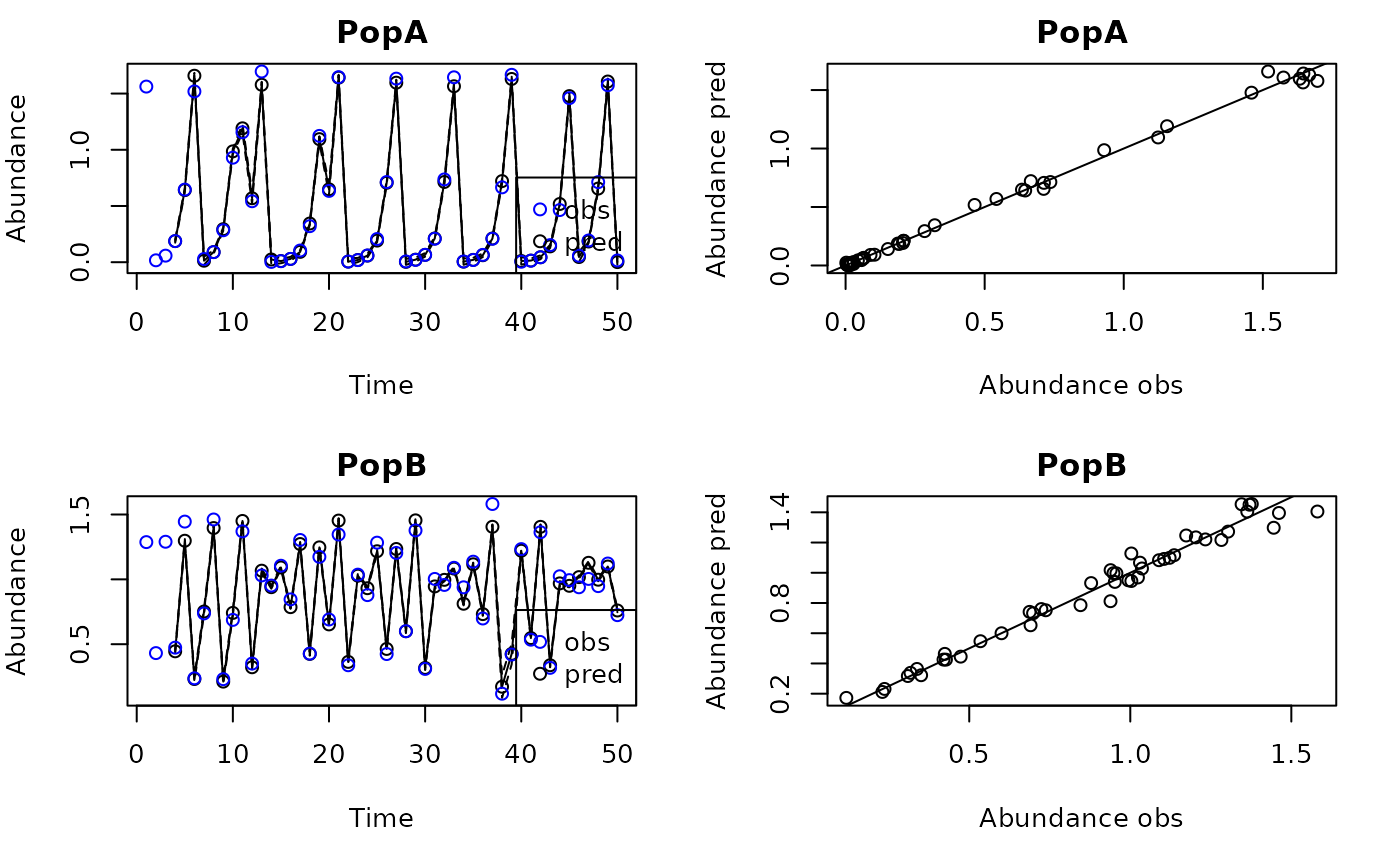

For more information on fitting hierarchical models, including the use of pairwise dynamic correlations with >2 populations, see this vignette.

Visualizing $f$ (conditional responses)

One thing you might be wondering is how we can visualize the shape of our fitted function $f$. If $f$ is 1- or 2-dimensional, we can create a grid of input values, pass them as newdata, and plot the resulting line or surface. If the function is more than 2 dimensional, this gets tricky, but we can look at slices of $f$ with respect to certain predictors, holding the values of the other predictors constant. The function getconditionals is a wrapper that will compute and plot conditional responses to each input variable with all other input variables set to their mean value. Although it does not show interactions, it can be useful for visualizing the effects of the predictors. Can also be used to check that your function isn’t doing something nonsensical and inconsistent with biology. To create 2-d conditionals surfaces, or to look at conditional responses with other predictors fixed to values other than their mean, you can pass an appropriately constructed grid to newdata. Visualizing models this way makes it possible to think about EDM from a more ‘mechanistic’ functional viewpoint.

#From the multivariate Hastings-Powell simulation
getconditionals(gp_out_mv)

Here are the conditional responses for the 2 population theta logistic simulation. Recall that the phi values for lags 2 and 3 were 0, so the corresponding relationship is flat.

#From the 2 population theta logistic
getconditionals(tlogtest)

Local slope coefficients from the GP

Just as with S-map, it is possible to obtain local slope coefficients from a GP model. The partial derivatives of the fitted GP function at each time point with respect to each input can be obtained from the predict function, setting returnGPgrad = T. They will be under model$GPgrad. The gradient will be computed for each out-of-sample prediction point requested (using methods "loo", "lto", or newdata). If you want the in-sample gradient, pass the original (training) data back in as newdata.

#From the multivariate Hastings-Powell simulation
grad1=predict(gp_out_mv2, predictmethod = "loo", exclradius = 6, returnGPgrad = T)
head(grad1$GPgrad)
#>       d_X_2      d_Y_2      d_Z_2
#> 1        NA         NA         NA
#> 2        NA         NA         NA
#> 3 0.8778238 -0.5689806 0.03631435
#> 4 0.8618503 -0.4125486 0.02126581
#> 5 0.9504046 -0.5375552 0.03520486
#> 6 0.9334179 -0.4231009 0.02623887

gradplot=cbind(HPtrain_lags_mv_train, grad1$GPgrad)

par(mfrow=c(3,1),mar=c(4,4,2,1))
plot(d_X_2~Time, data=gradplot, type="l")
plot(d_Y_2~Time, data=gradplot, type="l")
plot(d_Z_2~Time, data=gradplot, type="l")

Other things to know

You can, alternatively, pass the training/test data to the functions as vectors and matrices rather than in a data frame. This may make more sense if you’re doing simulations and just have a bunch of vectors and matrices, rather than importing data in a data frame.

The makelags function has some other bells and whistles you might want to check out, like creating matrix for forecasting beyond the end of a time series, and creating lags suitable for the variable step size method (more about that here).

There are a few additional, optional arguments to fitGP. initpars are the starting values of the hyperparameters, if for some reason you want to change those. modeprior is a value used in the phi prior that controls the expected number of modes the resulting function has over the unit interval (defaults to 1). Larger values for modeprior make the prior less informative. The only reason to change this would be to test whether the prior is having any influence on the results. linprior fits the model to the residuals of a linear relationship between y and the first variable of x. More information about this can be found in the fisheries vignette.