GPEDM Models For Fisheries
fisheries.RmdIntroduction
This vignette discusses the use of an alternative parameterization of
the GP-EDM model designed for use in fisheries applications, implemented
in the function fitGP_fish. This fits a GP model of the
form
where
is an index of abundance (typically in units of catch per unit effort,
CPUE),
are lags of
,
are lags of harvest (in biomass or numbers), and
are optional covariates. The index of abundance is assumed proportional
to biomass, with proportionality constant
(the “catchability”, units: CPUE/biomass). The composite variable
is assumed proportional to the biomass of individuals remaining after
harvesting (“escapement”).
The function fitGP_fish finds parameter
using stats::optimize applied to the posterior likelihood
of fitted GP models given
.
If you want to skip optimization of
and use a fixed value for it, one can be provided under
bfixed.
The function fitGP_fish has all of the same
functionality as fitGP, including the use of hierarchical
structures and augmentation data, and can be used with all of the
predict functions in the package. In all prediction cases,
it is only necessary to supply
and
- escapement will be calculated internally. The inputs and structure of
the inputs are somewhat more constrained than in fitGP (see
below), which is just something to be aware of.
Sample dataset
As a sample dataset, we will use a simulated Ricker model with harvest. This model has chaotic dynamics, and data from two ‘regions’. For this first example we will just use Region A, where we know the true value of is 0.01.
data("RickerHarvest")
RickerHarvestA=subset(RickerHarvest, Region=="A")
RickerHarvestB=subset(RickerHarvest, Region=="B")
par(mfrow=c(1,2),mar=c(4,4,2,1))
plot(Catch~Time, data=RickerHarvestA, type="l", main="Region A")
plot(CPUE_index~Time, data=RickerHarvestA, type="l", main="Region A")
Fitting a model
The function fitGP_fish requires the use of
data with pre-generated lags (option A1 in Specifying
training data)). Values for y, m, and
h are required, which should be the names of the
appropriate columns in data. A value for time
is also recommended. For the sample dataset, we will use just one
lag.
RHlags=makelags(RickerHarvestA, y=c("CPUE_index","Catch"), time="Time", tau=1, E=1, append=T)

fishfit0=fitGP_fish(data=RHlags, y="CPUE_index", m="CPUE_index_1", h="Catch_1", time="Time")
summary(fishfit0)
#> Number of predictors: 1
#> Fisheries model b: 0.01008
#> Length scale parameters:
#>         predictor posteriormode
#> phi1 escapement_1       1.08909
#> Process variance (ve): 0.03538059
#> Pointwise prior variance (sigma2): 2.978148
#> Number of populations: 1
#> In-sample R-squared: 0.9683622
Computed values of “escapement” (lagged) will be appended to the
model$insampresults table (also to any
model$outsampresults table). By default, the composite
variable will be called “escapement”, unless you supply a different name
for it (argument xname of fitGP_fish). In this
case, no data transformation is applied (see Data tranformations, so
predmean_trans and predmean are the same.
head(fishfit0$insampresults)
#>   timestep pop predmean_trans predfsd_trans predsd_trans obs_trans  predmean
#> 1        1   1             NA            NA           NA 15.074782        NA
#> 2        2   1      68.839049      1.070020     4.992834 64.075778 68.839049
#> 3        3   1       1.858803      2.948409     5.698822  1.987008  1.858803
#> 4        4   1      32.931192      2.021955     5.279371 30.573418 32.931192
#> 5        5   1      30.510587      1.235031     5.030781 31.422368 30.510587
#> 6        6   1      28.405921      1.193412     5.020726 28.992217 28.405921
#>         obs escapement_1
#> 1 15.074782           NA
#> 2 64.075778    14.922865
#> 3  1.987008    63.223627
#> 4 30.573418     1.969085
#> 5 31.422368    29.884448
#> 6 28.992217    30.866295
Conditional effects (from getconditionals) will be
plotted with respect to the calculated escapement values (and any
covariates, if present).
getconditionals(fishfit0)
Note that this function does not go through (0,0) because there are no data there. This could potentially cause problems if the model is extrapolated to regions of low or no escapement (as a result of high catch rates).
To force the model through the origin (so that zero escapement means
zero CPUE), you can supply an additional datapoint at 0 escapement, 0
CPUE. It works well to supply these under augdata, since
these points are used as training data and in determining the range the
conditional plots, but will not be included in the results table, used
to evaluate fit, or plotted as part of the time series. Note that the
model will probably not go through 0 exactly, because error is assumed
the same at the origin as it is elsewhere. Also note that if a
population experiences substantial immigration or emigration, the true
function may not actually intersect the origin.
#force zero escapement = zero CPUE
#the value for Time doesn't matter, but it should NOT be an NA
zeropin=data.frame(Time=0,CPUE_index=0,CPUE_index_1=0,Catch_1=0)

fishfit=fitGP_fish(data=RHlags, y="CPUE_index", m="CPUE_index_1", h="Catch_1", time="Time",
                   augdata=zeropin)
summary(fishfit)
#> Number of predictors: 1
#> Fisheries model b: 0.01007
#> Length scale parameters:
#>         predictor posteriormode
#> phi1 escapement_1       1.33691
#> Process variance (ve): 0.03383819
#> Pointwise prior variance (sigma2): 3.167774
#> Number of populations: 1
#> In-sample R-squared: 0.969906

getconditionals(fishfit)
Multiple populations
If you have multiple regions (populations), each with their own CPUE
index and Catch values, you can fit a hierarchical model using
fitGP_fish in the same way as fitGP. The
default behavior is to assume that
is the same for both population (bshared=TRUE). Supplying a
single value under bfixed will use the same fixed value for
all populations.
To estimate separate
values for each population, set bshared=FALSE. This will
use the Nelder-Mead method of stats::optim, which will be
quite a bit slower than the single
optimization, so more than 3 populations would not be recommended. You
can fix different values of
for each population by supplying a named vector under
bfixed.
If using different values of
,
be sure to use scaling="local" because the values are
assumed to be in different units by virtue of having different
catchabilities, but the dynamics should be proportional. You may want to
check whether the combined model actually produces better
within-population fits than the models fit separately. If there are
sufficient data, there is a good chance it will not.
The sample dataset contains time series for a second region B, where the true value of is 0.005. It also has a different catch history.
par(mfrow=c(1,2),mar=c(4,4,2,1))
plot(Catch~Time, data=RickerHarvestB, type="l", main="Region B")
plot(CPUE_index~Time, data=RickerHarvestB, type="l", main="Region B")
A separate model fith to region B:
#model for region B
RHlagsB=makelags(RickerHarvestB, y=c("CPUE_index","Catch"), time="Time", tau=1, E=1, append=T)
zeropin=data.frame(Time=0,CPUE_index=0,CPUE_index_1=0,Catch_1=0)

fishfitB=fitGP_fish(data=RHlagsB, y="CPUE_index", m="CPUE_index_1", h="Catch_1", time="Time",
                    augdata=zeropin)
summary(fishfitB)
#> Number of predictors: 1
#> Fisheries model b: 0.00471
#> Length scale parameters:
#>         predictor posteriormode
#> phi1 escapement_1       0.81279
#> Process variance (ve): 0.04297006
#> Pointwise prior variance (sigma2): 3.263646
#> Number of populations: 1
#> In-sample R-squared: 0.9609037
A hierarchical model assuming a single value:
RHlags2pop=makelags(RickerHarvest, y=c("CPUE_index","Catch"), time="Time",
                    pop = "Region", tau=1, E=1, append=T)
zeropin=data.frame(Region=c("A","B"),Time=0,CPUE_index=0,CPUE_index_1=0,Catch_1=0)

#model assuming a shared b
fishfit2pop1=fitGP_fish(data=RHlags2pop, y="CPUE_index", m="CPUE_index_1", h="Catch_1",
                        pop="Region", time="Time", scaling = "local", augdata = zeropin)
summary(fishfit2pop1)
#> Number of predictors: 1
#> Fisheries model b: 0.00492
#> Length scale parameters:
#>         predictor posteriormode
#> phi1 escapement_1       1.83144
#> Process variance (ve): 0.07313195
#> Pointwise prior variance (sigma2): 1.963022
#> Number of populations: 2
#> Dynamic correlation (rho): 0.9642383
#> In-sample R-squared: 0.9311925
#> In-sample R-squared by population:
#>          R2
#> A 0.9063203
#> B 0.9585102
A hierarchical model assuming separate values of (estimated):
#model assuming separate b values (takes a while to run)
fishfit2pop2=fitGP_fish(data=RHlags2pop, y="CPUE_index", m="CPUE_index_1", h="Catch_1",
                        pop="Region", time="Time", scaling = "local", augdata = zeropin,
                        bshared = FALSE)
summary(fishfit2pop2)
#> Number of predictors: 1
#> Fisheries model b:
#>          b
#> A 0.010015
#> B 0.004720
#> Length scale parameters:
#>         predictor posteriormode
#> phi1 escapement_1       0.91005
#> Process variance (ve): 0.03853103
#> Pointwise prior variance (sigma2): 3.298228
#> Number of populations: 2
#> Dynamic correlation (rho): 0.920653
#> In-sample R-squared: 0.9727368
#> In-sample R-squared by population:
#>          R2
#> A 0.9684365
#> B 0.9605205
A hierarchical model assuming separate values of (fixed):
#model assuming separate b values (fixed values)
b=c(A=0.01, B=0.005)
fishfit2pop2f=fitGP_fish(data=RHlags2pop, y="CPUE_index", m="CPUE_index_1", h="Catch_1",
                        pop="Region", time="Time", scaling = "local", augdata = zeropin,
                        bfixed = b)
summary(fishfit2pop2f)
#> Number of predictors: 1
#> Fisheries model b:
#>       b
#> A 0.010
#> B 0.005
#> Length scale parameters:
#>         predictor posteriormode
#> phi1 escapement_1       0.89022
#> Process variance (ve): 0.04024012
#> Pointwise prior variance (sigma2): 3.43141
#> Number of populations: 2
#> Dynamic correlation (rho): 0.9244014
#> In-sample R-squared: 0.9722251
#> In-sample R-squared by population:
#>          R2
#> A 0.9684097
#> B 0.9574334
getconditionals(fishfit2pop2f)
If more flexibility is required or you want to do something more
elaborate, below is code for how you could calculate escapement
externally given some value(s) of
,
and fit a regular fitGP to the escapement values. The
example below fits the same model as above (with
fixed).
bA=0.01
bB=0.005
RHlags$escapement_1=RHlags$CPUE_index_1-RHlags$Catch_1*bA
RHlagsB$escapement_1=RHlagsB$CPUE_index_1-RHlagsB$Catch_1*bB

par(mfrow=c(1,2),mar=c(4,4,2,1))
plot(CPUE_index~escapement_1, data=RHlags, main="Region A")
plot(CPUE_index~escapement_1, data=RHlagsB, main="Region B")
RHlagscombo=rbind(RHlags, RHlagsB)
zeropin=data.frame(Region=c("A","B"),Time=0,CPUE_index=0,escapement_1=0)

fishfitcombo=fitGP(data=RHlagscombo, y="CPUE_index", x="escapement_1", time="Time",
                   pop="Region", scaling="local", augdata=zeropin)
summary(fishfitcombo)
#> Number of predictors: 1
#> Length scale parameters:
#>         predictor posteriormode
#> phi1 escapement_1       0.89022
#> Process variance (ve): 0.04024012
#> Pointwise prior variance (sigma2): 3.43141
#> Number of populations: 2
#> Dynamic correlation (rho): 0.9244014
#> In-sample R-squared: 0.9722251
#> In-sample R-squared by population:
#>          R2
#> A 0.9684097
#> B 0.9574334
Getting MSY using iterated prediction
Given a fitted fisheries model, the steady state catch and biomass
given a certain harvest rate can be obtained using iterated prediction.
This can be done using the predict_iter function. Similar
to predict, you supply a newdata data frame,
which (for a one-population model) should contain the time,
m, and h columns. You also supply a harvest
rate hrate from 0 to 1, which indicates the proportion of
predicted CPUE biomass to be harvested.
Starting with the first row of newdata, the predicted
y variable is inserted into the first column of
m for the next timestep, and the other values of
m are shifted right by 1. The first value of h
at the next timestep is calculated as y/b*hrate and the
other values of h are shifted right by 1. Escapement is
recalculated, and a new prediction for y is made. This
continues for as many rows as are in newdata. Thus, this
procedure assumes that all lags are present, evenly spaced, and in order
(first lag is the first column). Time steps are assumed to be evenly
spaced. The units of y and m are assumed to be
the same.
In newdata, only the first timepoint (row) for
m and h needs to be filled in. The rest can be
NA and will be filled in as the model iterates forward. The values of
time must be filled in. If there are covariates
(z), they should also be included in newdata,
and values must be supplied for all time points. If there are multiple
populations, newdata should contain pop and
there should be duplicated timesteps for each population (see the next
sections for a 2-population example).
#number of timesteps to iterate
nfore=50

#use the forecast feature to create the first row
RHfore1=makelags(RickerHarvestA, y=c("CPUE_index","Catch"), time="Time", tau=1, E=1, forecast=T)
#get remaining timepoints. use expand.grid here if you have multiple populations.
RHfore2=data.frame(Time=(RHfore1$Time[1]+1):(RHfore1$Time[1]+nfore-1))
#create empty matrix for future values
RHfore3=matrix(NA, nrow=nrow(RHfore2), ncol=2,
               dimnames=list(NULL,c("CPUE_index_1","Catch_1")))
#combine everything
RHfore=rbind(RHfore1,cbind(RHfore2,RHfore3))

head(RHfore)
#>   Time CPUE_index_1  Catch_1
#> 1  101     22.36223 661.5723
#> 2  102           NA       NA
#> 3  103           NA       NA
#> 4  104           NA       NA
#> 5  105           NA       NA
#> 6  106           NA       NA
Since that is kind of annoying, I have written a wrapper for it
called makelags_iter. The arguments are the same as
makelags but you specify nfore and it makes
the matrix above.
RHfore=makelags_iter(nfore=50, data=RickerHarvestA, y=c("CPUE_index","Catch"),
                     time="Time", tau=1, E=1)
head(RHfore)
#>   Time CPUE_index_1  Catch_1
#> 1  101     22.36223 661.5723
#> 2  102           NA       NA
#> 3  103           NA       NA
#> 4  104           NA       NA
#> 5  105           NA       NA
#> 6  106           NA       NA
This matrix can be passed to predict_iter, specifying a
harvest rate.
msyfore=predict_iter(fishfit, newdata = RHfore, hrate = 0.5)The output of predict_iter can be passed to
plot if desired, which will plot CPUE (y). Note that there
will not be any observed values. The resulting escapement and catch
values will be included in the outsampresults table.
plot(msyfore)
#> Plotting out of sample results.
head(msyfore$outsampresults)
#>   timestep pop predmean_trans predfsd_trans predsd_trans predmean escapement_1
#> 1      101   1       66.63400      1.106339     4.929575 66.63400    15.697977
#> 2      102   1       23.73961      1.240739     4.961467 23.73961    33.317000
#> 3      103   1       73.60276      1.084414     4.924701 73.60276    11.869805
#> 4      104   1       18.54411      1.160412     4.941992 18.54411    36.801380
#> 5      105   1       74.34391      1.094346     4.926898 74.34391     9.272053
#> 6      106   1       18.02498      1.141830     4.937662 18.02498    37.171954
#>     Catch_1
#> 1  661.5723
#> 2 3307.4387
#> 3 1178.3370
#> 4 3653.3394
#> 5  920.4534
#> 6 3690.1269
For a given harvest rate, may be valuable to plot the projection alongside the past values.
#CPUE
ggplot(msyfore$outsampresults, aes(x=timestep, y=predmean)) +
  geom_line(size=1) + #iterated predictions
  geom_line(data=fishfit$insampresults) + ylab("CPUE") + #past predictions
  geom_point(data=fishfit$insampresults, aes(y=obs)) #observed values
#> Warning: Using `size` aesthetic for lines was deprecated in ggplot2 3.4.0.
#> ℹ Please use `linewidth` instead.
#> This warning is displayed once every 8 hours.
#> Call `lifecycle::last_lifecycle_warnings()` to see where this warning was
#> generated.
#> Warning: Removed 1 row containing missing values or values outside the scale range
#> (`geom_line()`).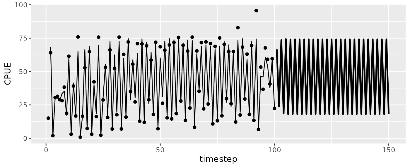
#Catch
ggplot(msyfore$outsampresults, aes(x=timestep, y=Catch_1)) +
  geom_line(size=1) +
  geom_line(data=RHlags, aes(x=Time)) #past catches
#> Warning: Removed 1 row containing missing values or values outside the scale range
#> (`geom_line()`).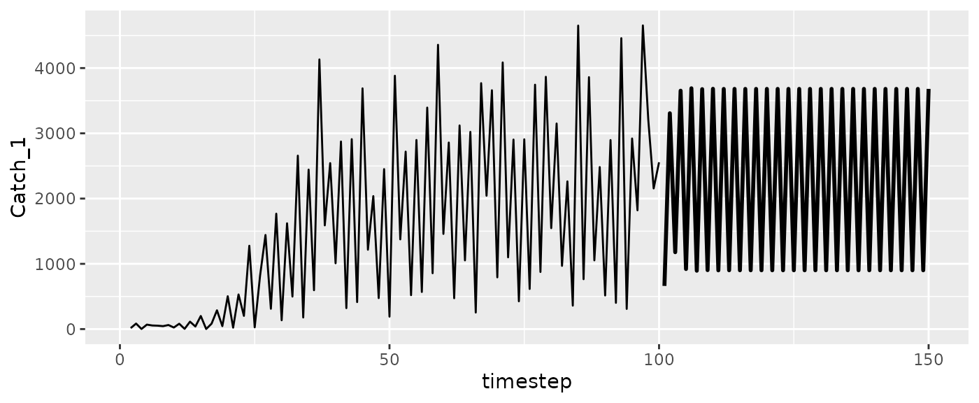
#Escapement
ggplot(msyfore$outsampresults, aes(x=timestep, y=escapement_1)) +
  geom_line(size=1) +
  geom_line(data=fishfit$insampresults) #past escapements
#> Warning: Removed 1 row containing missing values or values outside the scale range
#> (`geom_line()`).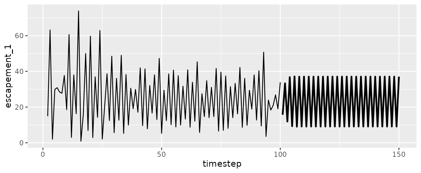
Evaluating the steady state catch across a range of
hrate values allows you to obtain the maximum sustainable
yield (MSY), associated fishing rate (f_MSY), and associated CPUE
indexed biomass (proportional to B_MSY). In the example below, we make
iterated predictions for 50 timesteps as above, but record just the last
10 values. Since the resulting time series in this example can exhibit
chaos and cycles, we then take the average over those values for each
harvest rate.
#vector of harvest rates
hratevec=seq(0,1,length.out=30)
#number of timepoints to save
tsave=10

catchsave=expand.grid(time=1:tsave,hrate=hratevec)
catchsave$catch=NA
catchsave$cpue=NA
for(i in seq_along(hratevec)) {
  msyfore=predict_iter(fishfit, newdata = RHfore, hrate = hratevec[i])
  #note that the next 2 lines only work if there is one population
  catchsave$catch[catchsave$hrate==hratevec[i]]=
    msyfore$outsampresults$Catch_1[(nfore-tsave+1):nfore]
  catchsave$cpue[catchsave$hrate==hratevec[i]]=
    msyfore$outsampresults$predmean[(nfore-tsave+1):nfore]
}

#average over the last 10 timepoints
catchsavemean=aggregate(cbind(catch,cpue)~hrate, data=catchsave, mean)
(fmsy=catchsavemean$hrate[which.max(catchsavemean$catch)])
#> [1] 0.862069
(Bmsy=catchsavemean$cpue[which.max(catchsavemean$catch)])
#> [1] 74.7035

par(mfrow=c(1,2),mar=c(4,4,2,1))
plot(catch~hrate, data=catchsave, col="gray")
lines(catch~hrate, data=catchsavemean, lwd=2, col="red")
abline(v=fmsy, col="red")
plot(cpue~hrate, data=catchsave, col="gray")
lines(cpue~hrate, data=catchsavemean, lwd=2, col="red")
abline(v=fmsy, col="red")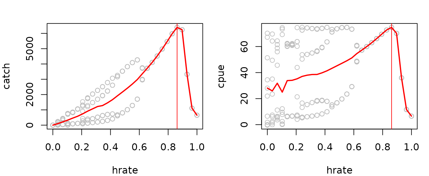
Here’s a wrapper for all of that as well. Since there is only one
population here, the ‘total’ and ‘pop’ output tables are identical. The
ones you really care about are catchforeall which are all
the predictions, catchsavetotal which are the last
tsave predictions, and catchsavetotalmean
which is the average of the last tsave predictions.
hratevec=seq(0,1,length.out=30)
msyout=msy_wrapper(model=fishfit, newdata = RHfore, hratevec = hratevec, tsave = 10)
msyout$fmsy
#> [1] 0.862069
msyout$Bmsy
#> [1] 74.7035

par(mfrow=c(1,2),mar=c(4,4,2,1))
plot(catch~hrate, data=msyout$catchsavetotal, col="gray")
lines(catch~hrate, data=msyout$catchsavetotalmean, lwd=2, col="red")
abline(v=msyout$fmsy, col="red")
plot(cpue~hrate, data=msyout$catchsavetotal, col="gray")
lines(cpue~hrate, data=msyout$catchsavetotalmean, lwd=2, col="red")
abline(v=msyout$fmsy, col="red")
Let’s look at the trajectory for the population at fmsy.
#you can get this either by rerunning predict_iter
msytraj=predict_iter(fishfit, newdata = RHfore, hrate = fmsy)$outsampresults
#or if you have used the msy_wrapper, you can get it out or the catchforeall table
msytraj=subset(msyout$catchforeall, hrate==fmsy)

#CPUE
ggplot(msytraj, aes(x=timestep, y=predmean)) +
  geom_line(size=1) + #iterated predictions
  geom_line(data=fishfit$insampresults) + ylab("CPUE") + #past predictions
  geom_point(data=fishfit$insampresults, aes(y=obs)) #observed values
#> Warning: Removed 1 row containing missing values or values outside the scale range
#> (`geom_line()`).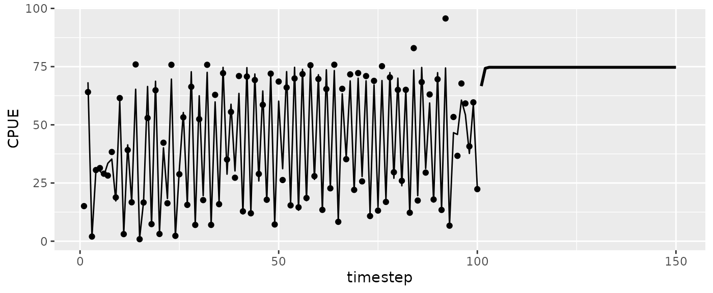
#Catch
ggplot(msytraj, aes(x=timestep, y=Catch_1)) +
  geom_line(size=1) +
  geom_line(data=RHlags, aes(x=Time))
#> Warning: Removed 1 row containing missing values or values outside the scale range
#> (`geom_line()`).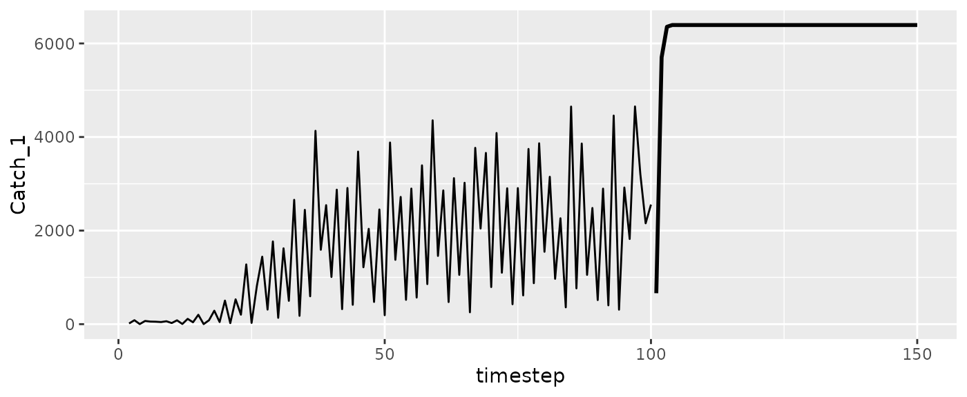
#Escapement
ggplot(msytraj, aes(x=timestep, y=escapement_1)) +
  geom_line(size=1) +
  geom_line(data=fishfit$insampresults)
#> Warning: Removed 1 row containing missing values or values outside the scale range
#> (`geom_line()`).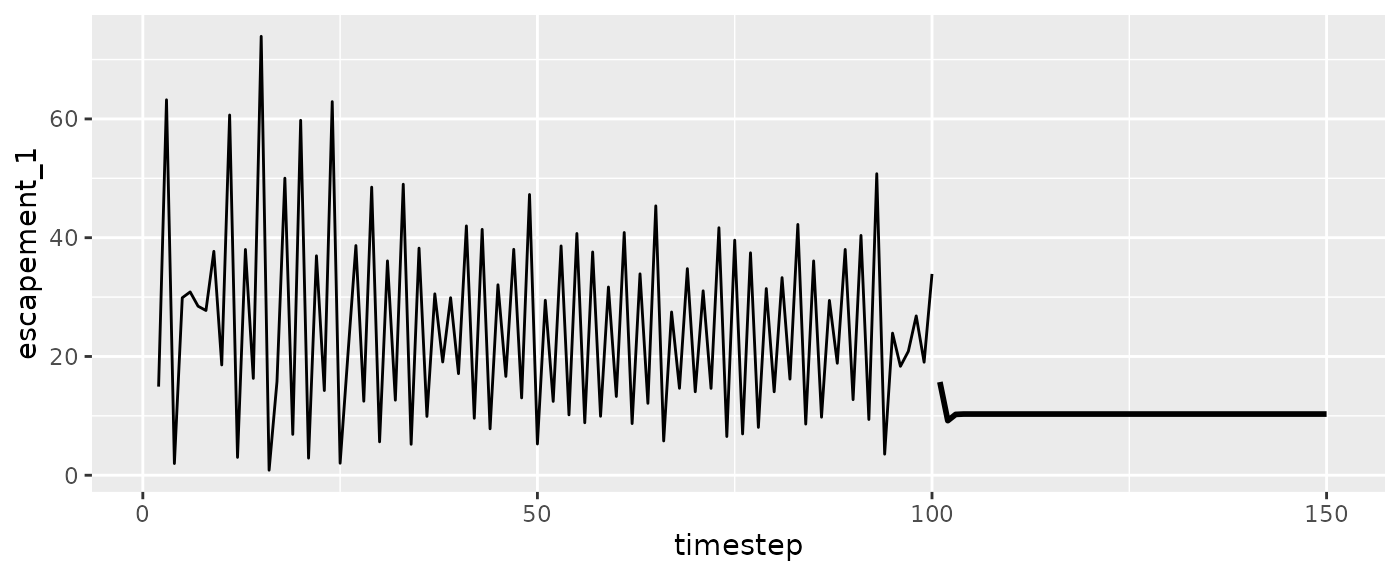
Let’s compare this to the true analytical solution for this model using the simulation parameters.
r=3; K=1000
q=0.01 #catchability b
tbiomass=K/(1-hratevec)*(r-log(1/(1-hratevec))) #steady state biomass
tcpue=q*tbiomass
tcatch=hratevec*tbiomass

par(mfrow=c(1,2),mar=c(4,4,2,1))
plot(catch~hrate, data=msyout$catchsavetotalmean, type="l", lwd=2, col="red")
lines(tcatch~hratevec, lwd=2, col="cornflowerblue")
abline(v=msyout$fmsy, col="red")
legend(x="topleft", legend = c("EDM","true"), col=c("red","cornflowerblue"), lwd=2, cex=0.8)
plot(cpue~hrate, data=msyout$catchsavetotalmean, type="l", lwd=2, col="red")
lines(tcpue~hratevec, lwd=2, col="cornflowerblue")
abline(v=msyout$fmsy, col="red")
legend(x="topleft", legend = c("EDM","true"), col=c("red","cornflowerblue"), lwd=2, cex=0.8)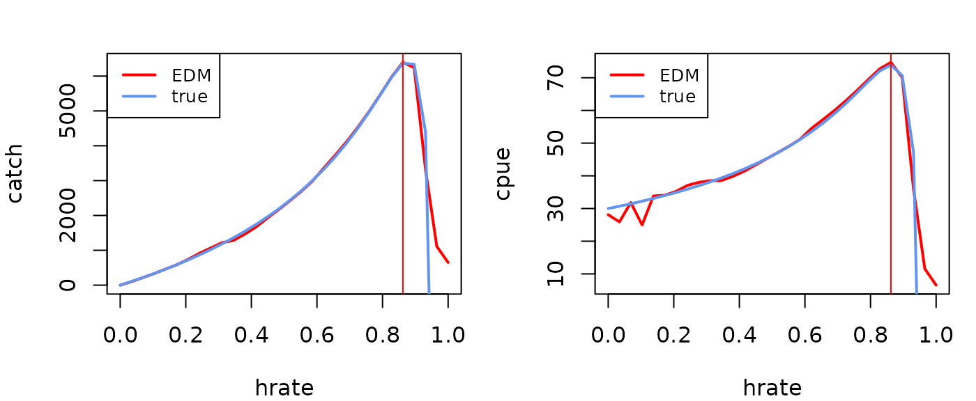
It is also possible to set this up using a constant catch value
rather than constant catch rate. To do this, omit hrate and
fill all the catch rows and columns in newdata with a
constant value. In this example with chaotic dynamics, this can lead to
negative escapement, so it was not done here.
MSY with multiple populations
If you have a multi-population fitGP_fish model that
assumes a single values of
,
or if you are using separate fitGP_fish models for each
population, you should be able to use predict_iter as
above, but will need to keep track of the predictions for each
population and decide if you want to add them together or not.
At present, the harvest rate is assumed the same for all populations. This may change in the future.
#make the forecast matrix
RHfore2pop=makelags_iter(nfore=50, data=RickerHarvest, y=c("CPUE_index","Catch"),
                         time="Time", tau=1, E=1, pop="Region")
head(RHfore2pop)
#>   Time Region CPUE_index_1   Catch_1
#> 1  101      A     22.36223  661.5723
#> 2  101      B     31.04974 3854.1177
#> 3  102      A           NA        NA
#> 4  103      A           NA        NA
#> 5  104      A           NA        NA
#> 6  105      A           NA        NA
Plots of the trajectories for a given harvest rate:
msyfore2pop=predict_iter(fishfit2pop2, newdata = RHfore2pop, hrate = 0.5)
head(msyfore2pop$outsampresults)
#>   timestep pop predmean_trans predfsd_trans predsd_trans predmean escapement_1
#> 1      101   A       67.20451     1.0805364     5.238766 67.20451     15.73647
#> 2      101   B       22.21612     0.7308345     2.627487 22.21612     12.85822
#> 3      102   A       23.57338     1.1304705     5.249293 23.57338     33.60225
#> 4      102   B       25.68929     0.7574316     2.635009 25.68929     11.10806
#> 5      103   A       74.26029     1.0231498     5.227232 74.26029     11.78669
#> 6      103   B       22.24372     0.7311363     2.627571 22.24372     12.84464
#>     Catch_1
#> 1  661.5723
#> 2 3854.1177
#> 3 3355.1344
#> 4 2353.3919
#> 5 1176.8833
#> 6 2721.3100

#CPUE
ggplot(msyfore2pop$outsampresults, aes(x=timestep, y=predmean, color=pop, group=pop)) +
  geom_line(size=1) +
  geom_line(data=fishfit2pop2$insampresults) + ylab("CPUE") +
  geom_point(data=fishfit2pop2$insampresults, aes(y=obs))
#> Warning: Removed 2 rows containing missing values or values outside the scale range
#> (`geom_line()`).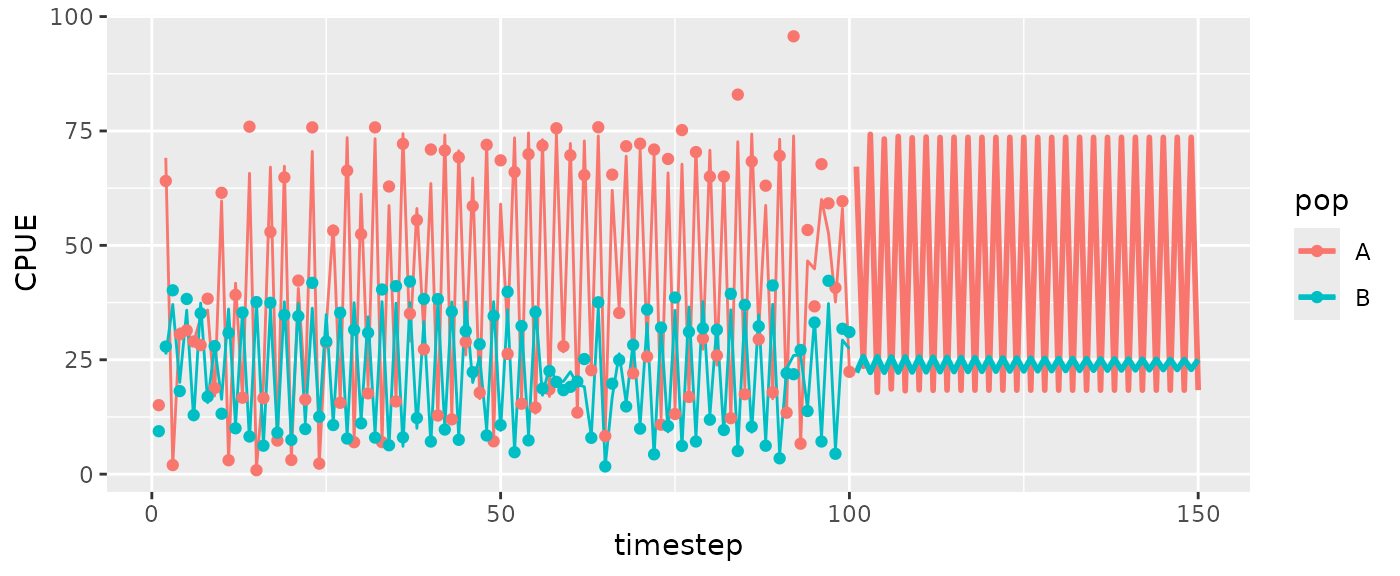
#Catch
ggplot(msyfore2pop$outsampresults, aes(x=timestep, y=Catch_1, color=pop, group=pop)) +
  geom_line(size=1) +
  geom_line(data=RHlags2pop, aes(x=Time, color=Region, group=Region))
#> Warning: Removed 2 rows containing missing values or values outside the scale range
#> (`geom_line()`).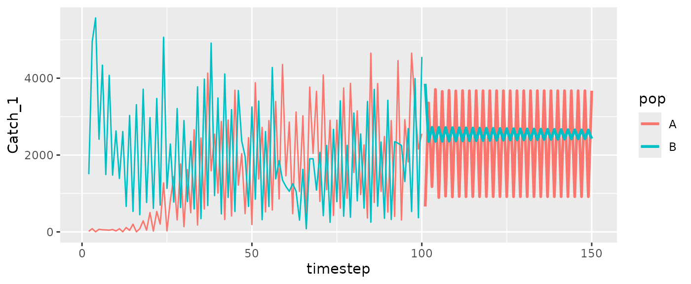
#Escapement
ggplot(msyfore2pop$outsampresults, aes(x=timestep, y=escapement_1, color=pop, group=pop)) +
  geom_line(size=1) +
  geom_line(data=fishfit2pop2$insampresults)
#> Warning: Removed 2 rows containing missing values or values outside the scale range
#> (`geom_line()`).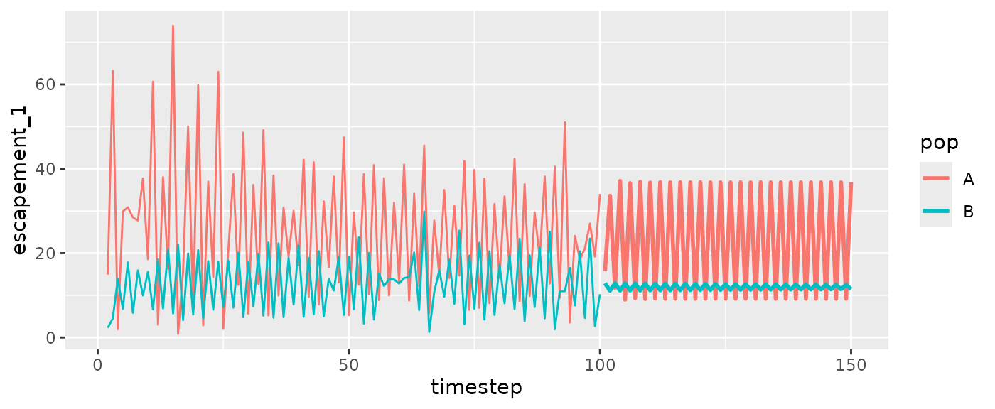
Evaluate a grid of harvest rates to obtain MSY using the wrapper.
Since there are multiple populations, the ‘total’ and ‘pop’ tables will
be different. The MSY estimates reported by the function are based on
catchsavetotalmean, but you could compute population
specific estimates if desired.
hratevec=seq(0,1,length.out=30)
msyout2pop=msy_wrapper(model=fishfit2pop2, newdata = RHfore2pop, hratevec = hratevec, tsave = 10)
msyout2pop$fmsy
#> [1] 0.862069
msyout2pop$Bmsy
#> [1] 112.3226

#Total
par(mfrow=c(1,2),mar=c(4,4,2,1))
plot(catch~hrate, data=msyout2pop$catchsavetotal, col="gray")
lines(catch~hrate, data=msyout2pop$catchsavetotalmean, lwd=2, col="red")
abline(v=msyout2pop$fmsy, col="red")
plot(cpue~hrate, data=msyout2pop$catchsavetotal, col="gray")
lines(cpue~hrate, data=msyout2pop$catchsavetotalmean, lwd=2, col="red")
abline(v=msyout2pop$fmsy, col="red")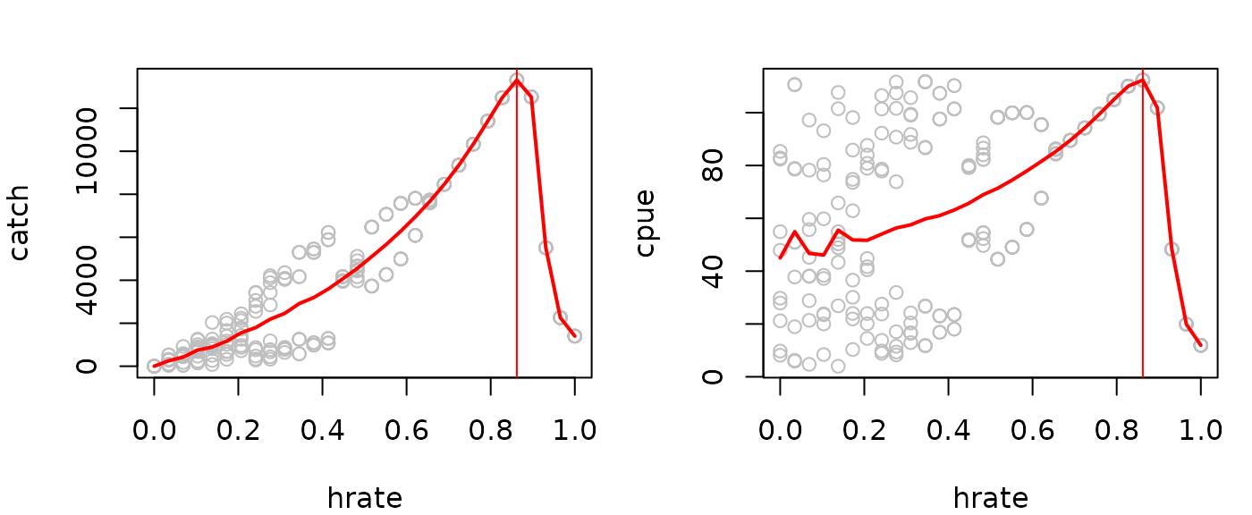
#Split up by pop
ggplot(msyout2pop$catchsavepop, aes(x=hrate, y=catch, color=pop)) +
  geom_point(alpha=0.5) +
  geom_line(data=msyout2pop$catchsavepopmean, size=1) +
  geom_vline(xintercept = msyout2pop$fmsy, color="black")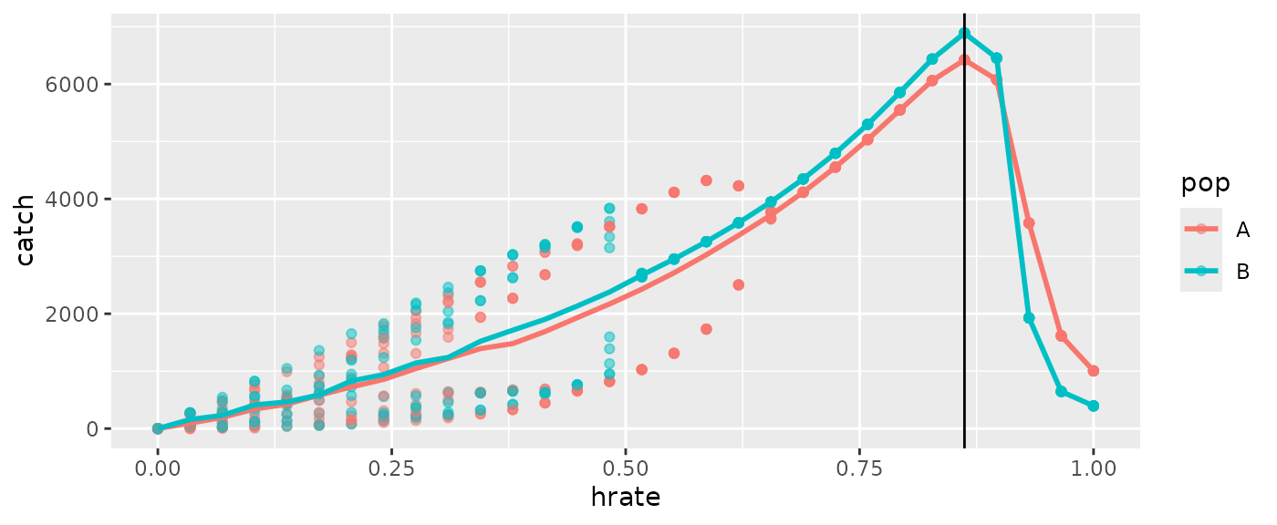
ggplot(msyout2pop$catchsavepop, aes(x=hrate, y=cpue, color=pop)) +
  geom_point(alpha=0.5) +
  geom_line(data=msyout2pop$catchsavepopmean, size=1) +
  geom_vline(xintercept = msyout2pop$fmsy, color="black")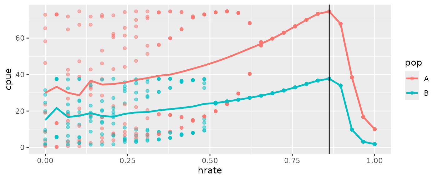
If you are computing escapement externally, you will probably have to
write a custom loop, like below. This is mostly the internal code of
predict_iter but with some modification.
#calculate escapement
RHfore2pop$b=ifelse(RHfore2pop$Region=="A", bA, bB)
RHfore2pop$escapement_1=RHfore2pop$CPUE_index_1-RHfore2pop$Catch_1*RHfore2pop$b

head(RHfore2pop)
#>   Time Region CPUE_index_1   Catch_1     b escapement_1
#> 1  101      A     22.36223  661.5723 0.010     15.74651
#> 2  101      B     31.04974 3854.1177 0.005     11.77915
#> 3  102      A           NA        NA 0.010           NA
#> 4  103      A           NA        NA 0.010           NA
#> 5  104      A           NA        NA 0.010           NA
#> 6  105      A           NA        NA 0.010           NA

#vector of harvest rates
hratevec=seq(0,1,length.out=40)
#number of timepoints to save
tsave=10

#rename some stuff to minimize recoding
popname="Region"
timename="Time"
object=fishfitcombo
xlags="CPUE_index_1"
hlags="Catch_1"
newtimes=unique(RHfore2pop[,timename])
up=unique(RHfore2pop[,popname])

#setup final data frame
catchsavepop=expand.grid(pop=up,time=1:tsave,hrate=hratevec)
catchsavepop$catch=NA
catchsavepop$cpue=NA

pred=list()

for(h in seq_along(hratevec)) {

  newdata=RHfore2pop
  hrate = hratevec[h]

  #iterated prediction loop
  for(i in seq_along(newtimes)) {
    newdatai=newdata[newdata[,timename]==newtimes[i],]
    #get prediction
    pred[[i]]=predict(object, newdata=newdatai)$outsampresults
    preds=pred[[i]]
    #create new data row for each population
    #assumes all lags are present and evenly spaced
    if(i+1 <= length(newtimes)) {
      for(j in 1:length(up)){
        predsj=preds[preds$pop==up[j],]$predmean
        thisrowj=newdata[,timename]==newtimes[i] & newdata[,popname]==up[j]
        nextrowj=newdata[,timename]==newtimes[i+1] & newdata[,popname]==up[j]
        newdata[nextrowj,xlags[1]]=predsj
        if(length(xlags)>1) {
          newdata[nextrowj,xlags[2:length(xlags)]]=newdata[thisrowj,xlags[1:(length(xlags)-1)]]
        }
        #compute next catch
        newdata[nextrowj,hlags[1]]=predsj/newdata[nextrowj,"b"]*hrate
        if(length(xlags)>1) {
          newdata[nextrowj,hlags[2:length(xlags)]]=newdata[thisrowj,hlags[1:(length(xlags)-1)]]
        }
      }
      #compute escapement
      newdata$escapement_1=newdata[,xlags]-newdata[,hlags]*newdata[,"b"]
    }
  }

  #combine results
  msyfore=do.call(rbind, pred)
  msyfore=cbind(msyfore,newdata[,hlags,drop=F])

  #pull out last tsave timepoints for each population
  for(p in 1:length(up)){
    msyforei=subset(msyfore, pop==up[p])
    nfore=nrow(msyforei)
    catchsavepop$catch[catchsavepop$hrate==hratevec[h] & catchsavepop$pop==up[p]]=
      msyforei[(nfore-tsave+1):nfore,hlags[1]]
    catchsavepop$cpue[catchsavepop$hrate==hratevec[h] & catchsavepop$pop==up[p]]=
      msyforei$predmean[(nfore-tsave+1):nfore]
  }
}

#sum over pops (if more than one)
catchsavetotal=aggregate(cbind(catch,cpue)~hrate*time, data=catchsavepop, sum)

#average over the last 10 timepoints (keeping split by pop)
catchsavepopmean=aggregate(cbind(catch,cpue)~hrate*pop, data=catchsavepop, mean)

#average over last 10 timepoints (sum of pops)
catchsavetotalmean=aggregate(cbind(catch,cpue)~hrate, data=catchsavetotal, mean)

(fmsy=catchsavetotalmean$hrate[which.max(catchsavetotalmean$catch)])
#> [1] 0.8717949
(Bmsy=catchsavetotalmean$cpue[which.max(catchsavetotalmean$catch)])
#> [1] 111.6516
Data transformations
The argument ytrans in fitGP_fish can be
used to apply a data transformation to y prior to fitting
the model. Inputs y and m should always be in
untransformed CPUE. Setting ytrans="none" (the default)
will apply no tranformation, ytrans="log" with compute
,
ytrans="gr1" will compute
,
and ytrans="gr2" will compute
.
All
values will be computed in the original (untransformed) units of CPUE.
Note that the standard deviations in the results table are only for the
transformed variable.
The conditional responses (from getconditionals) will
plot the transformed variable. The plot method will plot
the untransformed variable (without standard deviations), unless you
specify ytrans=TRUE.
fishfit0_trans=fitGP_fish(data=RHlags, y="CPUE_index", m="CPUE_index_1", h="Catch_1", time="Time",
                          ytrans="gr2")
summary(fishfit0_trans)
#> Number of predictors: 1
#> Fisheries model b: 0.00981
#> Length scale parameters:
#>         predictor posteriormode
#> phi1 escapement_1       0.01457
#> Process variance (ve): 0.003093382
#> Pointwise prior variance (sigma2): 4.082601
#> Number of populations: 1
#> In-sample R-squared: 0.9700048

head(fishfit0_trans$insampresults)
#>   timestep pop predmean_trans predfsd_trans predsd_trans   obs_trans predmean
#> 1        1   1             NA            NA           NA          NA       NA
#> 2        2   1     1.51840279    0.01277130   0.09303044  1.45690654 68.13988
#> 3        3   1    -3.36206912    0.03390825   0.09819025 -3.46039904  2.19232
#> 4        4   1     2.74031519    0.02511391   0.09551055  2.74232496 30.51203
#> 5        5   1     0.01032261    0.01321373   0.09309221  0.04958110 30.21267
#> 6        6   1    -0.09053364    0.01318509   0.09308814 -0.06310678 28.20786
#>         obs escapement_1
#> 1 15.074782           NA
#> 2 64.075778    14.924034
#> 3  1.987008    63.230185
#> 4 30.573418     1.969223
#> 5 31.422368    29.889751
#> 6 28.992217    30.870574

getconditionals(fishfit0_trans)![]()
plot(fishfit0_trans)
#> Plotting in sample results.![]()
plot(fishfit0_trans, ytrans = TRUE)
#> Plotting in sample results.![]()
Linear prior mean function
There is an option in fitGP (and
fitGP_fish) called linprior which will fit a
GP model to the residuals of a linear relationship between
y and the first variable of x (prior to
scaling) and backtransform as appropriate. Essentially, it fits the
model
where
is the GP. In other words, the mean function for the GP is assumed to be
linear with respect to the first input, rather than constant. The mean
function is what the GP reverts to in the absence of data (the larger
the inverse length scale is, the more quickly this happens), so altering
it can potentially aid in problems with extrapolation. In a fisheries
model, if y is growth rate (specifically the
escapement-based growth rate, "gr2"), the first variable of
x will be the first lag of escapement, and so this linear
relationship at acts like a Ricker prior. Option
linprior="local" fits a separate regression for each
population, "global" fits a single regression. Defaults to
"none" (off).
In our example, the fitted function looks largely the same. The
difference between this and the previous fit is mainly in what happens
when you extrapolate beyond the range of the data. We can see it in the
conditional response plot is we set extrap to a high
number.
fishfit0_lin=fitGP_fish(data=RHlags, y="CPUE_index", m="CPUE_index_1", h="Catch_1", time="Time",
                          ytrans="gr2", linprior = "global")
getconditionals(fishfit0_trans, extrap = 1)
getconditionals(fishfit0_lin, extrap = 1)