Practical considerations when using EDM with real data

library(GPEDM)

Introduction

There are some practical considerations and decisions one needs to make when applying EDM to real data (as opposed to simulated). This vignette covers an assortment of these considerations. Since we work on population dynamics, we’ll mostly be referring to the data as ‘abundance’ but know that this generalizes to other types of data.

In short, because the dynamics of real data, unlike simulated data, are unknown, there is likely going to be more experimentation and exploration involved in finding the best and most appropriate model. For any given system, the default modeling choices are not necessarily going to be the best ones. If you find that EDM doesn’t work that well on the first pass, it is worth thinking about the theory and why it might not be working. Consider things like the natural history of your organism, the amount of data you have, the level of observation noise, the ‘observation function’ created by the sampling method, the sampling interval of the time series, and other topics that are discussed in more detail below. This might give you some insight into alternative structures that could improve performance. There are frequently modifications that can be made that can improve prediction accuracy.

First things first: How much data is do I need?

Because EDM is data-driven, it would be inadvisable to attempt it on anything with less than about 30 data points, simply because there will not be enough data to empirically reconstruct an attractor. If you have individual time series that are too short, but you have multiple replicates (so the total number of data points is higher), that can help alleviate this issue, as long as the replicates have similar underlying dynamics and are not highly synchronized (in which case, they wouldn’t be adding any additional information). However, depending on the time scales of dynamics in your system, and on the sampling interval, you may need quite a bit more than 30 data points to effectively reconstruct dynamics.

To empirically quantify system dynamics in general, the time series length needs to be several multiples of the “characteristic return time” for the system. The characteristic return time is the time it takes for the system state to return to a small neighborhood of a given starting state. In other words, the time series needs to have “recurrences” (multiple visits to similar states), so that past trajectories can actually be used to forecast future trajectories. If a time series has no or too few recurrences, there will not be enough useful neighbors from past trajectories to follow, no matter how high the sampling frequency is.

When it comes to real data, the generation time of the organism is often a good proxy for the characteristic return time. For example, Munch et al. (2018) found that when time series length was 10 times the mean age at maturation, EDM could explain >50% of the variation in recruitment in several fish species. For short-lived species, there is often a significant in prediction error when we have >30 years of data (Sugihara et al. 2012; Ye et al. 2015; Munch et al. 2018). For long-lived organisms like whales or redwood trees, unless you have centuries worth of data, EDM might not be the best tool. Over the short term, the dynamics of long-lived organisms are likely to be dominated by inertia (autocorrelation), and there may be no recurrences.

If your data are periodic or semi-periodic and show population cycles, then the dominant period can also be a good proxy for the characteristic return time. For short-lived organisms undergoing a seasonal cycle, you will probably need data over several cycles (years).

Time series length and sampling interval will pose some limitations on your ability to reconstruct the deterministic dynamics. The maximum embedding dimension that can be recovered is roughly equal to the square root of the time series length (Cheng and Tong 1992). Thus, if the attractor dimension is large and the time series is short, we expect a fair amount of unexplained variation (prediction error) to remain, because the additional dimensions are non-recoverable given the available data. Also, if the dynamics are occurring on time scales much shorter than the sampling interval, they will be difficult to reconstruct and lead to apparent indeterminism.

Pro-tip #1: Plot your data

This may seem obvious, but always plot your time series before fitting any models. This goes for simulated data as well, but is especially important for empirical data. You would be surprised how many people fail to do this. Plotting the data can quickly reveal potential issues that could trip up EDM. For example, your time series could have one giant outlier, be 90% zeros, be constant for long time periods, be smoothed/interpolated but only for the first half, have a huge gap in the middle, be monotonically increasing, etc. Being familiar with your data will help guide your decisions as far as data preparation before fitting models and help you understand what results you’re getting.

If you’re using a database with hundreds or thousands of time series, you can automate some filtering out of inappropriate time series by setting criteria for length, missing values, zeros, etc. You may still end up with a lot of series, and well, you should still plot them all. The following code allows you to plot them 12 at a time, pressing enter to move to the next set.

# 'myseries' are your time series in long format, with columns ID, Time, Abundance
IDs=unique(myseries$ID)
par(mfrow=c(4,3),mar=c(4,4,2,1))
for(i in IDs) {
  plot(Abundance~Time, data=subset(myseries, ID==i), main=i, type="o")
  if(which(IDs==i)%%12==0) {
    readline(prompt="Press [enter] to continue")
  }
}

Steve likes to create a movie where each time series displays for 10 seconds or less, which is plenty of time to spot problems.

Pro-tip #2: Know your goal

Also before fitting any models, think about what your goal is. Knowing your research questions or objectives can help guide the choices you make. Are you making a tactical forecast model for use by managers? In that case, you really want to maximize forecast performance and tailor a very specific model. Are you interested in ecological inference? In that case you need to think carefully about the model structure and interpretability. Takens’ shows there are many possible representations of a dynamical system, and the ‘best’ model for one goal may not be the ‘best’ model for another goal.

Data Processing

By data processing, we are referring to treatment of the data prior to fitting any models. Note that there is no one ‘right’ way to process your data, and you may have to explore a few options to find what works best for your system. Many of these questions to ask yourself are common to all types of time series analyses, not strictly EDM.

Do I transform my data?

Takens’ theorem applies not only to the original state variables, but also to observation functions (including transformations) of those those state variables, provided they still span the full attractor space. So it is perfectly fine to transform your data, and certain transformations might make it easier for the EDM algorithms to reconstruct the dynamics because they spread the points out in a more useful way for identifying/weighting neighbors and obtaining the next state.

Data transformation (e.g. log transformation) matters practically for EDM because it affects the Euclidean distances between points (and thus their weighting). The nearest neighbors on one scale are not necessarily the nearest neighbors on another scale.

Ecological abundance data are often lognormally distributed and “spikey”, appearing more periodic when log transformed. In EDM, it is often (but not always) the case that squashing the high values closer together through a log transformation makes the attractor easier to model and produces better predictions, in part because the “spikes” are closer and more likely to have useful neighbors. Plotting your data (untransformed vs. transformed) can give you a good sense of whether this is likely to be the case.

Data transformation can also be important if you want to ensure that your predictions are confined to certain values (e.g. non-negative values). If there are many data values close to zero, EDM can potentially produce negative abundance forecasts, which may be undesirable (note that average-based function approximations like Simplex can never do this, but others methods can). Log-scale predictions, when backtransformed, will always produce positive numbers. Logit transforms, $\log(y/(1-y))$ , may also be similarly desirable for data constrained between 0 and 1.

In parametric modeling, one reason we typically do data transformation is to meet assumptions about the distribution of residuals. Non-parametric models, like those used in EDM, vary in their assumptions about the distribution of residuals, so the choice to do a data transformation may also be informed by the EDM method you are using, and what your goals are. Nearest neighbor and local linear approaches minimize sums of squares without necessarily assuming normality, but GP approaches assume Gaussian distributed residuals. However, violating these assumptions only matters if you want to interpret the confidence or credible intervals around the means or the coefficients, or conduct ‘significance tests’. This is not typically done in EDM, so unlike parametric models, these assumptions usually aren’t tested or worried about much. That said, if your data are highly non-Gaussian, you should consider data transformations to avoid a small handful of outliers having undue influence on the results. This goes for all EDM methods, not just the GP.

Another thing to consider is what to use as your “response variable” or “target”. In standard, univariate EDM, the target and its lag predictors are the same variable and all on the same scale and in the same units. But this need not necessarily be the case. The target and/or predictors could be abundance, log abundance, first differenced abundance ( $y_{t+1}-y_{t}$ ), log growth rate ( $ln(y_{t+1})-ln(y_t)$ , equivalently $ln(y_{t+1}/y_{t})$ ), or some other transformation. You can mix and match. If $Y_t=ln(y_t)$ , the following are a few of the many possible valid EDM formulations:

$\begin{aligned} y_{t+1}&=f(y_{t},y_{t-1},...,y_{t-E}) \\ Y_{t+1}&=f(Y_{t},Y_{t-1},...,Y_{t-E}) \\ y_{t+1}-y_{t}&=f(y_{t},y_{t-1},...,y_{t-E}) \\ y_{t+1}-y_{t}&=f(y_{t}-y_{t-1},y_{t-1}-y_{t-2},...,y_{t-(E-1)}-y_{t-E}) \\ Y_{t+1}-Y_{t}&=f(y_{t},y_{t-1},...,y_{t-E}) \\ Y_{t+1}-Y_{t}&=f(Y_{t},Y_{t-1},...,Y_{t-E}) \\ \end{aligned}$

So how do you know which is best for your system? See the section below on model selection. If abundance and log abundance don’t look very different, then you can probably just pick one of them. If you’re trying to select among models with different transformations of the response variable, you will probably want to backtransform all of the predictions to the original units and re-evaluate fit, so that the fits for all models are based on the same set of values and therefore comparable. Backtransforming and re-evaluating fit is also a good idea if what you actually care about are forecasts in the original units (e.g. real fish, not log fish or fish population growth rate). The model that maximizes fit to the transformed data may not be the same one that maximizes fit in the original units.

What do I do with zeros?

Log transforming zeros

If you decide to do a log transformation, you’ll invariably end up with a the time series with zeros in it, which of course cannot be log transformed. What do you do in this annoying situation? You could decide to use a square root transformation instead. If you really want to stick with the log transformation though, then you could add a small value to all of the data points prior to transforming them. However, you should be very cautious when doing this. You might think it totally reasonable to add a tiny value like 0.0001, that is basically zero, but look how it distorts the distances in the figure below. Using EDM on this time series would not be recommended. If your data are integers and include reasonably low non-zero values, adding 1 might be a better choice. If the the lowest non-zero values is something like 1000, then you might want to add 1000, or whatever the minimum non-zero value is. Plotting the transformed time series is highly recommended to check that the distortion at low values is not too great for whatever you decide to do.

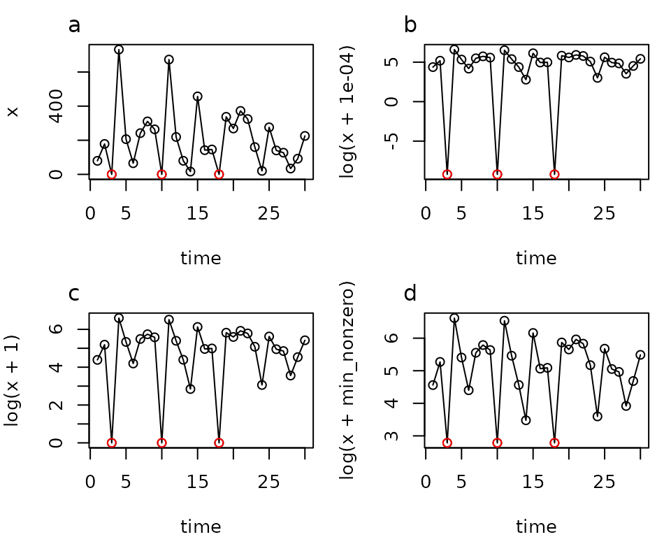
$\label{fig:logtrans2} Log transforming data with zeros. Varying amounts of distortion occur when adding different values. The minimum non-zero value in this time series is 16.2. Zeros are plotted in red. The time series is a sequence of lognormal random values (mean 5, sd 1) with 3 zeros manually added.$

Log transforming data with zeros. Varying amounts of distortion occur when adding different values. The minimum non-zero value in this time series is 16.2. Zeros are plotted in red. The time series is a sequence of lognormal random values (mean 5, sd 1) with 3 zeros manually added.

Too many zeros

If your time series has a lot of zeros in it (e.g. more than half of data are zeros) that is concerning for other reasons. Most likely, it is not because there are actually zero organisms (which in a closed system would mean permanent extinction), but rather that abundance is lower than some detection threshold, or that the organisms have moved out of the sampling area (e.g. migration), or the organisms are in some life history stage where you can’t sample them (e.g. resting stages, seeds, small individuals that pass through your net). This is not in itself a problem as far as EDM theory - you can think of it as an observation function (applied by your sampling method) to actual abundance, but it is something to be aware of. If the observation function does not allow you to see the full attractor because it squashes a lot of values to the origin, then EDM is not likely to work very well (or it will work deceivingly great, because all the predictions are just zero). For this reason, we generally avoid doing EDM of series with a high proportion of zeros.

The ‘too many zeros’ problem can sometimes be solved by aggregating spatial replicates or coarsening the time resolution, so that your observation function encompasses more space and/or time, if sufficient replication exists and this makes sense for your system (see section below on aggregation).

For species that are present seasonally but absent for most of the rest of the year (zero or not sampled at all because abundance is known to be zero), you could try a peak-to-peak type of map, which may work well if you have data from enough seasons. Annual averaging is another option. Or, you could fit two maps: One for the short steps during the period where the species are typically present and a second map to jump over the season when they are absent.

Should I standardize my data?

In GPEDM, the priors are based on the assumption that the predictor and response variables are centered and scaled, so they should be standardized. However, fitGP will standardize (and back-standardize) the inputs internally, so standardizing them beforehand will not make a difference. Also, because GPEDM has separate inverse length scales for each coordinate, standardization in mixed (multivariate) embeddings is less critical than it is for EDM algorithms. This is because the weighting can be different (and optimized) along each axis.

Standardizing matters and gets more complicated if you have replicate time series because you can choose to standardize either within series (use local mean and standard deviation) or across series (use global mean and standard deviation). Both can be reasonable approaches depending on the particular system and sampling design, and is worth putting some thought into it because standardizing within vs. across series can lead to very different model fits and performance. With replicates, you are assuming that the time series come from the same (or a similar) attractor, and by combining them, you can get a more complete picture of it. Standardizing within replicates could overlay different parts of the attractor on top of each other that should actually be separated. On the flip side, if each replicate is a differently scaled version of the attractor, overlaying them without standardizing will not create a clear picture of the attractor. In both cases, you won’t be able to identify useful neighbors.

As a simple example, consider the effect of temperature on population growth rate of a species, where you have data from several sites across a temperature (e.g. latitudinal) gradient, where the real relationship is unimodal (highest at intermediate temperatures). Combining data from across sites, you could see this relationship if you standardized temperature across sites, allowing each site to retain different local means. However, if you centered and scaled all the temperatures within sites, removing their local means, it would likely just look like a mess, and you might conclude that cold populations have a completely different response to temperature than warm populations (one increasing, the other decreasing), when really it is just one shared unimodal response.

Generally speaking, if the variable has the same units across series, you will probably want to use “global” standardization. If the variable has different units, you will probably want to use “local” standardization. However, you may have valid reasons to deviate from this, and trying both might be worthwhile if in doubt. For instance, if a species of interest has different carrying capacities in different regions but the same underlying dynamics, local standardization of each region might make more sense, even if the units are the same. If you have covariates, you might choose to use different standardizations for different variables (e.g. local standardization of abundance, but global standardization for temperature). These choices matter for all EDM algorithms.

One should standardize data after applying transformations. You can’t take the log after something has been centered on zero.

Note: With other EDM algorithms (simplex, s-map), if you are only using univariate time lags from a single time series, the results should be identical whether you standardize that time series or not. This is because standardization (a linear transformation) does not change the relative distances among points in delay coordinate space (it just moves the whole attactor sideways, and scales it larger or smaller). Plus for simplex and s-map, the distances among points are actually standardized internally (it is built into the weighting kernel), so that the weighting kernel operates the same way regardless of the range of the data. Standardizing does matter when using mixed coordinates (multivariate predictors) because they are in different units, and simplex and s-map (unlike GP-EDM) weight neighboring points equally in all directions. If a covariate (for instance) has a way bigger or smaller variance than than the abundance lags, then the attractor is going to stretched or squashed along that axis. This may not be ideal, which is why it’s often recommended to standardize all variables when mixing coordinates like this.

Should I detrend my data? What do I do about non-stationarity?

If your data has a monotonic trend with time, you should think about whether or not you want to keep or remove it. The answer is not always so clear cut.

If your series is completely dominated by a monotonic trend, and any deviations from that trend are just noise, EDM will not offer many advantages over simpler modeling approaches, and may not even be the best tool to use. If the trend (linear or otherwise) is removed and noise is all that is left, then EDM obviously will not perform very well because all the determinism is gone. In this case, you might just want to model the trend directly (abundance a function of time). If the trend is retained and the population is simply undergoing exponential growth or decay, then the best EDM will probably end up being just a 1-d linear model.

The typical argument for removing trends is to remove “nonstationarity”. Imagine the entire attractor moving in one direction over time due to some external driver. If this is really what is happening, then subtracting the trend (linear or otherwise) from the all abundance time series, as has been proposed in some papers, makes some sense, and you’ll be able to recover recurrences that would not otherwise be there.

However, there are plenty of stationary nonlinear systems with periods of high and low oscillations, that can appear to have a trend (or multiple “regimes”) if you’re only looking at a relatively short time series. This isn’t to say that nonstationarity isn’t a real issue for ecology, just that some apparent nonstationarity may instead reflect complexity and dynamics that play out over different time scales. In these cases, distorting distances by detrending could be removing important information about the dynamics, particularly if you’re combining a series with other replicates covering different parts of the attractor.

Whether to remove the trend also depends on what your goals are. If the trend is important and you care about actual abundance (rather than just abundance anomalies) you probably want to retain the trend, and ideally find something to explain it, whether that be internal dynamics or an external driver.

If you suspect your dynamics are influenced by a trend in an external driver (typically some aspect of ‘the environment’), there are a few approches one could take that don’t involve detrending the data. If you know what the driver is, the driver can simply be included as one of the coordinates. If you don’t know what the driver is, but are only making short-term predictions, and the system is changing slowly relative to the time scale of prediction, EDM on its own may work just fine: As long as the system behavior doesn’t change qualitatively in response to the driver, the recent past will still be a good proxy for the near future. If the system is changing more quickly, one could take advantange of time delays as proxies for unobserved variables (in this case, the driver) by simply adding more time lags - an approach known as over-embedding (Kantz and Schreiber 2003) that can account for nonstationarity. There are also variants of EDM that allow the nonlinear function to change over time (Munch et al. 2017), or that model the driver as a latent variable (Verdes et al. 2006) that could be explored, if desired.

One way to sidestep this problem is to use first differences or log growth rates rather than abundance, which tend to result in series that look more ‘stationary’. k-th order differencing removes k-th order trends in time, which could be really handy. However, it also amplifies noise, which could be problematic.

Should I smooth my time series?

In general, smoothing is not recommended, since it can “hide” deterministic features of the dynamics and create artifacts. For instance, if you smooth or interpolate large gaps using an ARIMA model, and find that your time series dynamics are linear, is that because they’re really linear, or is it because the ARIMA model has made them linear? Nonlinear dynamics can create ‘non-smooth’ temporal patterns, which will be lost if attributed to observation error and smoothed over. Smoothing is going to make things seem more linear than they might actually be.

While we’re on the topic of models imposing dynamics, this is also something you need to beware of when analyzing ‘data’ that is not actually raw data, but model output. Many abundance time series you find out in the world are not actually direct estimates of abundance, but the output of population dynamics models that have been fit to some data (of variable quantity and quality), usually with a lot of assumptions. These time series often look exceptionally smooth, and/or are constant for long periods (usually in the far past when there are no actual data), and a look into the metadata will often reveal that they come from a model. Analyzing these sorts of series with EDM is not recommended because of the dynamics imposed by the underlying model. EDM might just be recovering the Ricker or other model that was chosen, rather than the actual natural dynamics. For example, we were once looking at a set of time series from the North American Breeding Bird Survey, which can be found in the Living Planet Index Database, which all looked (when plotted) exceptionally smooth and suspiciously like either exponential growth or decay. Some digging revealed that all these series were from models of annual deviations imposed on growth trend. So, it’s no wonder they look mostly like exponential growth/decay because this behavior is built in to the model output! Suffice it to say, we did not analyze these, and EDM would no doubt conclude the dynamics are linear and 1-dimensional. Many (but not all) of the fish time series in the Ransom Myers’ Stock Recruitment Database are also model output, and need a closer look before you choose to analyze them.

If you know that your data have a lot of observation noise, you might want to use a Kalman filter in combination with EDM (Esguerra and Munch 2024), rather than smoothing. The underlying dynamics in this case are modelled using EDM, but with an added observation model.

Should I aggregate space? time? species? replicates?

This very much depends on the data, your question, and the scale at which you want to make predictions. Aggregation is good at fixing the problem of too many zeros and can reduce the amount of observation error, leading to more predictable dynamics. But too much aggregation might hide dynamics occurring at smaller scales that you might care about. As an extreme example, annually averaging monthly data won’t give you any information about seasonal dynamics. Aggregating data for individual species by functional group is common, in part because of the too many zeros problem, and this can also make the dynamics more predictable. However, it may hide other properties. For example, aggregates were found to be more dynamically stable than species-level series in plankton (Rogers et al. 2023).

How do I deal with missing data?

EDM algorithms (though not the underlying theory) typically assume the timesteps (each row in your data table) are evenly spaced. This means the following things will definitely screw up EDM:

Failure to insert missing timepoints
Duplicate values at a given timepoint
Timepoints not in chronological order
Multiple series stacked end to end without taking into account where one ends and the next starts

This is because when you go to construct lags, algorithms will find t-1 by looking 1 row up. If 1 row up is actually something else because of one of the problems above, your t-1 predictor will be t-1 sometimes, but occasionally t-something else.

Frequently, missing timepoints are omitted from raw data files and need to be inserted as missing values (NAs). For example:

#a monthly dataset with a lot of missing values
mydata <- data.frame(Year=c(2014,2014,2014,2014,2014,2014,2014,
                            2015,2015,2015,2015,2015,2015,2015),
                     Month=c(1,4,5,6,8,9,11,
                             1,2,5,6,7,8,12),
                     Abundance=round(rnorm(14,10,5)))
mydata
#>    Year Month Abundance
#> 1  2014     1        17
#> 2  2014     4         9
#> 3  2014     5        12
#> 4  2014     6        10
#> 5  2014     8         3
#> 6  2014     9         8
#> 7  2014    11         8
#> 8  2015     1        10
#> 9  2015     2        16
#> 10 2015     5        14
#> 11 2015     6         9
#> 12 2015     7         9
#> 13 2015     8        13
#> 14 2015    12        13

alltimepoints <- expand.grid(Year=unique(mydata$Year), Month=1:12)

mydatafilled <- merge(alltimepoints, mydata, all.x = T)
mydatafilled
#>    Year Month Abundance
#> 1  2014     1        17
#> 2  2014     2        NA
#> 3  2014     3        NA
#> 4  2014     4         9
#> 5  2014     5        12
#> 6  2014     6        10
#> 7  2014     7        NA
#> 8  2014     8         3
#> 9  2014     9         8
#> 10 2014    10        NA
#> 11 2014    11         8
#> 12 2014    12        NA
#> 13 2015     1        10
#> 14 2015     2        16
#> 15 2015     3        NA
#> 16 2015     4        NA
#> 17 2015     5        14
#> 18 2015     6         9
#> 19 2015     7         9
#> 20 2015     8        13
#> 21 2015     9        NA
#> 22 2015    10        NA
#> 23 2015    11        NA
#> 24 2015    12        13

Once you have identified missing time points, you have to decide what to do with them. You have several options:

Keep them in and skip them: This will result in $E\tau$ datapoints being lost after every missing value. If there are not many missing values relative to the number of data points, this is probably fine. If there is one big gap in the time series, this is probably also a good option.
Interpolate: If your time series is fairly smooth and the missing data gaps are small and few in number, it may be completely reasonable to interpolate. This could be as simple as linear interpolation, or you could fit an EDM interpolation model that uses lags of the past and future to predict points in the middle, which may work better for less smooth series.
Use variable time step size EDM: This variant of EDM includes the time step between lags as an additional predictor. More detail about this method is provided here, and in Johnson and Munch (2022).

If you have missing data that is missing on a regular schedule (a common case would be that there is monthly sampling, but no sampling occurs for a few months in the middle of winter), you could be potentially justified in removing the missing values and treating the ‘gap’ as a single timestep. In the case of no winter sampling due to low abundance, inhospitable sampling conditions, or the ecosystem being literally frozen, this might make sense if you think there is not much change occurring during this period, or the dynamics are dramatically slowed in the ‘winter’ part of the cycle (likely to be the case for ectotherms). As mentioned earlier, missing data due to seasonally low (or zero) abundance could also be dealt with using annual averaging, peak to peak methods, or multiple models.

Model fitting

Evaluating model performance

Which performance metric should I use?

A measure of model performance is necessary to assess how well a given model fits the data, and also to compare performance among different candidate models. There are many different ways to quantify the difference between the model predicted values and the observed values. Which metric you choose will depend a bit on what your goals are.

Mean squared error (MSE) and root mean squared error (RMSE) are some of the most common error metrics, and in most model-fitting algorithms, the sum or squared errors (SSE, where MSE and RMSE come from), is what is being minimized.

$MSE=\frac{1}{n} \sum_{i=1}^n{(\hat{y_i}-y_i)^2}$

The $R^2$ value (proportion of the variance in $y$ explained by the model) is the MSE standardized by the observed variance, specifically

$R^2=1-\frac{SS_{error}}{SS_y}=1-\frac{MSE}{Var(y)}$

This means a few things:

For different models of the same time series, RMSE and $R^2$ are inversely related. Note, if you’re working with standardized time series where $Var(y)=1$ , then $1-MSE = R^2$ .
The magnitude of $R^2$ is comparable across time series, whereas RMSE is not. This also applies to different subsets of the same time series.
The $R^2$ can be negative if the predictions are worse than the mean (the MSE exceeds the variance in $y$ ). This will never happen with in-sample predictions from linear models, because the model is guaranteed to pass through the mean: the lowest the $R^2$ can ever be is 0, which will be from a constant model where the prediction equals the mean. However, when you are predicting out-of-sample (and also in certain nonlinear models), the model is not guaranteed to pass through the mean, and you can get negative $R^2$ values. If you get a negative $R^2$ , this is a sign that your model is not doing a good job, which might not be obvious just looking at RMSE alone.

All of these reasons are why we tend to prefer $R^2$ or another form of standardized error over unstandardized forms.

The correlation coefficient between the predicted and observed values ( $r$ ) is also frequently seen in the literature. You might think that $r$ is just the square root of $R^2$ , but it is not. It is true that $r^2=R^2$ for in-sample predictions from ordinary least squares, but this is not true for out-of-sample predictions or certain nonlinear models, where the model is not guaranteed to pass through the mean and you can have bias in the predictions.

More precisely, $r^2\geq R^2$ . This means that using $r$ can sometimes make model performance look better than it actually is, and that if there is strong bias, $r$ can be positive even when $R^2$ is negative.

Mean absolute error, $MAE=\frac{1}{n} \sum_{i=1}^n{|\hat{y_i}-y_i|}$ , and mean absolute percent error, $MAPE=\frac{1}{n} \sum_{i=1}^n{|(\hat{y_i}-y_i)/y_i|}$ , are less common, but can also be seen in the forecasting literature. They differ from MSE in the weight given to errors in various directions. For strictly positive data, percent error will penalize overforecasts more than underforecasts, because while there is a lower bound on the percent error for an underforecast, there is no upper bound on the percent error for an overforecast. The log accuracy ratio, $log(\hat{y}/y)$ , is another metric that has been proposed that penalizes over and under predictions evenly (Satterthwaite & Shelton 2023). Double or half the predicted value would be given equal weight by this metric.

If you’ve transformed the data, all of these performance metrics could be evaluated either on the transformed scale or on the original scale. Error calculated on the log scale will penalize deviations at high values less than deviations at low values, relative to the arithmetic scale.

In terms of which metric to use, particularly for tactical forecast models, you need to think about what is most important to get right in your forecast, or rather, what is the cost of being wrong in different ways. Are overforecasts worse than underforecasts? Is it more important to get high values right or low values right? Is accuracy more important on the log or arithmetic scale? How important is bias? The answers to these questions will depend on what is being forecast and how it is being used. You could potentially design your own performance metric specific to your needs and do model selection using that.

What level of performance is considered “good” depends a bit on your baseline. $R^2$ values tend to be higher for physical and physiological data than for ecological data, since ecological data tend to be shorter, more coarsely sampled, and to have more observation error. An $R^2$ above 0.5 for ecological data is considered quite good. If, despite your best efforts, you are unable to find a model with acceptable performance ( $R^2$ is less than 0.2 for instance) it may be that the time series available are insufficient to resolve much deterministic dynamics. For short ecological time series, this may happen. In those cases, it is probably better not to draw any conclusions or inferences from that model. Trusting forecasts from a model with low performance also wouldn’t be recommended; however, if the alternative model (e.g. the one currently used by managers) is even worse when using the same performance evaluation scheme and metric, then even a poorly performing model might be an upgrade.

How do I do model selection?

The most straightforward and reliable way to do model selection is to do out-of-sample cross-validation. This means that whatever point being predicted should not be included in the training data used for the model. As the model is made more complex and flexible, the in-sample model performance will always increase, but the out-of-sample performance will plateau and potentially start to decline due to overfitting. Thus, it is particularly important that EDM model fits be evaluated out-of-sample rather than in-sample. The model(s) to select will be the ones that maximize out-of-sample performance.

Model selection based on likelihoods (penalized by the model degrees of freedom) is common in parametric modeling (e.g. AIC), and can be done with the nonparametric models used in EDM (the degrees of freedom being approximated the trace of the smoother matrix). In theory, the out-of-sample performance and penalized likelihood should give consistent answers, but in practice this is not always the case. The penalized likelihood approach has some assumptions built in about the error distribution, and one can get potentially misleading answers if these assumptions are violated. Out-of-sample cross-validation is robust to a wide range of assumption violations, and so it is a better approach to use than penalized likelihood. The predictions must be genuinely out-of-sample though, and it also requires that you have sufficient data to get a reliable answer.

How do I choose a cross-validation scheme?

There are many (possibly infinite) ways to do out-of-sample cross-validation. Which one you choose is going to depend partly on how much data you have, and also what your goals are. The absolute performance of the models generally will change depending on which scheme you choose, because it becomes ‘harder’ to predict as you restrict the amount of training data available. However, the relative performance of models is likely not going to change much, which is important to keep in mind. If you are trying to choose the best among a set of models that all have acceptable (not poor) performance, then the answer will likely not be sensitive to your choice of cross-validation scheme.

If you have a good amount of data, spliting the data into a training and testing set is a common approach. You may find that performance results differ depending on the train/test split used, particularly if certain subsets of the time series contain extreme values, or very different variances. If this is a concern, you might consider a k-fold cross validation procedure that leaves out various chunks of the dataset.

Leave-one-out cross-validation (predictmethod="loo") is a popular for short datasets where training/testing splits are not realistic, and where there is not high serial autocorrelation. This is likely to be the case for most ecological data that are sampled on a fairly coarse time scale. For data with strong serial autocorrelation, such as that sampled on a fine temporal resolution or that are very smooth, leave-one-out is possible, but it is important to leave out not just the focal point from the training data, but also points on either side (temporally) of the focal point. This is referred to as the ‘Thieler window’ or ‘exclusion radius’(argument exclradius). The window/radius is typically $E\tau$ (for a fixed tau) or the maximum $\tau$ if using variable $\tau$ values. If this additional exclusion is not done, then the leave-one-out predictions are not genuinely out-of-sample, because the target point is (effectively) still in the training data, and performance estimates may be inflated.

Leave-one-out with replicate series also requires some consideration. If replicates are highly synchronized, then leaving a point out of one series may not truly be ‘removing’ it from the training data, if the same point exists (effectively) in another time series. Leaving out all points at a given time step might be a better option in this case (predictmethod="lto").

For tactical forecasting models, the ‘leave-future-out’ method is a popular approach. Here, for a portion of the time series (e.g. the last 20 timepoints, or the last 10%), forecasts are made using only the data preceding each point as training data. So, it is similar to the train/test split, but with multiple ‘splitting’ points. This simulates a real-time forecasting application where future is unknown, and what the forecasts would have been had they been made in the past using this model (function predict_seq).

One important thing to keep in mind (more relevant to leave-one-out than train/test, but still potentially problematic), is the relationship between $E\tau$ and data loss. The first $E\tau$ data points in a time series (and after every missing value if missing values are retained and skipped), will be lost as testing points, because they lack complete predictor information. So if you are evaluating different values of $E$ and $\tau$ , inconsistencies can arises due to the variable amounts of data being lost as $E$ and $\tau$ change, which for short test time series, can result in substantial changes to the baseline variance of the values being predicted across candidate models. This is especially problematic if there are more extreme abundance values just at the beginning of the time series. To avoid this, you will want to standardize the set of target points being tested to ones that can be estimated by all models. Poor or strange results can also be obtained if the test dataset is too short or has insufficient variance.

What should my forecast horizon be?

For any deterministic system, knowing the current state gives you enough information to predict all future states. However, in practice, things like noise, chaos, etc. prevent us from making predictions arbitrarily far into the future. In chaotic systems, as well as linear stochastic ones, we expect forecast accuracy to decline with increasing forecast horizon.

At the same time though, the forecast horizon should not be too small, particularly when dealing with high frequency data. If it is too short, $y$ hasn’t had the chance to change much, and best model will be inevitably be a linear model with $E=1$ (thus leading to the inescapable conclusion that all dynamics are linear). If the sampling interval is short relative to the system dynamics, you should try evaluate performance over a longer (though still reasonable) horizon, or over multiple time horizons, either directly or through iteration.

In terms of software implementations, a common model structure is to have the forecast horizon equal to the time delay $\tau$ , such that the prediction and the time lags are evenly spaced,

$y_t=f(y_{t-\tau},y_{t-2\tau},...,y_{t-E\tau})$

or equivalently,

$y_{t+\tau}=f(y_{t},y_{t-\tau},...,y_{t-(E-1)\tau})$

but this need not necessarily be the case. The forecast horizon can also be set independently.

$y_{t+h}=f(y_{t},y_{t-\tau},...,y_{t-(E-1)\tau})$

or equivalently

$y_{t}=f(y_{t-h},y_{t-\tau-h},...,y_{t-(E-1)\tau-h})$ What you choose for the forecast horizon $h$ depends on your question, sampling interval, and the time scale over which you are aiming to make predictions.

Selecting hyperparameters

How do I choose $E$ and $\tau$ ?

See this entire other vignette for information on choosing embedding parameters, with some worked examples.

Mixing lags (multiple $\tau$ values)

Many EDM implementations (and software packages) assume a single value of $\tau$ resulting in evenly spaced time lags, $\tau, 2\tau,...,E\tau$ . But this need not necessarily be the case. It is completely allowable to mix time lags, $\tau_1, \tau_2,...,\tau_E$ ,

$y_t=f(y_{t-\tau_1},y_{t-\tau_2},...,y_{t-\tau_E})$

For example, instead of using all 12 time lags from 1 to 12, you could use just 1, 2, and 12. Such an approach often works well for series with dynamics happening on multiple time scales, e.g. inter-annual and intra-annual dynamics. Dropping unneeded time lags reduces the embedding dimension, allowing for additional degrees of freedom, and potentially more accurate predictions. In GP-EDM, the dropping of uninformative lags by ARD achieves effectively uneven time lags automatically. In other methods that require a grid search, allowing for uneven lags introduces yet another layer of factorial combinations, which in combination with multiple predictors that can have uneven lags, can start to look pretty daunting. In these cases, EDM approaches have been developed that use random combinations of predictors and time lags, and combine them using model averaging.

If your goal is inference, it is probably more important to find an interpretable model rather than the best possible model for forecasting, so you may want to use a fixed model structure with a limited set of candidate models, particularly if you’re applying it to a large number of time series. If your goal is tactical forecasting for a single time series, you may want to do more exploration of alternate structures and lag spacing, and dive more into maximizing forecast performance. Knowledge of the biology of the system can be applied to help choose reasonable candidate models.

How do I deal with seasonality?

Seasonality is very common in ecological data sampled sub-annually. There are a few possible ways you can deal with it.

You could do nothing, and allow the time lags to take care of it. In this case, you probably want to consider lags that are the length of the cycle (12 months) in the set of candidate models. Models with a mix of short and long lags to account for inter-annual and intra-annual dynamics might we worth trying.
You could include a seasonal predictor in the model. Note that since seasonality is a cycle, the seasonal predictor needs to be 2-dimensional (a circle, though 1-d, needs to be embedding in a 2-d Euclidean space). For instance, you could use a sine and a cosine function with periods of 12 months. This approach may be useful for inference, e.g. if you want to control for seasonal effects when estimating species interactions. It might also help in terms of forecast performance.
You could remove seasonality by substracting the monthly mean, for instance, and modeling seasonal anomalies. This poses some of the same issues as detrending the data, but may be appropriate and improve performance in some cases.

Seasonality poses some particular issues when using CCM to assess causal linkages. If you have a number of variables that are all entrained in a seasonal cycle, you can get some strange and erroneous results from CCM, e.g. that disease incidence drives environmental temperature. Disentangling the influence of a common seasonal driver from an actual interaction can be tricky. The ‘seasonal surrogates’ approach is one method that attempts to separate the effect of seasonality from that of other dynamics. Ultimately, our ability to resolve this depends on how much internal dynamics exist independently of seasonality. If none, there may still be directional causal relationships between variables, but reliably determining them from time series alone becomes impossible.

Inconsistency, ambiguity, and getting the ‘right’ answer

Takens’ shows there are many possible representations of a dynamical system, and so many models (particularly with multivariate predictors) can have equivalent performance. Some models will ‘work’ better than others, and the best model may differ depending on your goal. Many people worry about getting the ‘right’ values of $E$ and $\tau$ , but since there is no ‘right’ answer, we suggest not worrying too much about this, and thinking more about your goal.

If you’re wanting to make inference based on performance, the hyperparameters (e.g. $E$ , the inverse length scales), the local slope coefficients/gradient, or other derived quantities, more care needs to be taken in terms of model structure and selection. If you have multivariate data, it’s important to be mindful of the ability of time lags to compensate for missing state variables. For instance, if you are trying to evaluate the effect of an environmental driver, but that driver is already accounted for by the time lags, adding the driver will lead to no improvement in performance, and it will appear as if the driver has no effect. Dropping lags and seeing if the driver continues to have no effect might be a solution. As another example, it becomes very challenging to interpret the local slope coefficients from lag predictors because they incorporate many indirect effects as well as potentially unobserved variables, and don’t necessarily reflect a direct effect of e.g. lag $t-3\tau$ from species A on species B. Interpreting the coefficients from just the first (or most recent) lags might be more appropriate. Particularly for inference studies, your results should ideally be robust to minor differences in $E$ , and you may want to conduct sensitivity analyses.

If what you care about is forecasting, the model struture is less of a concern, though you may still want to eliminate models that are completely inconsistent with known biology. You also have to consider practicalities like data availability. You might find that $y_{t-1}$ is an excellent predictor of $y_t$ , but if $y_{t-1}$ isn’t available at the time you need to be making a prediction, then that model is functionally useless, and you need to explore other models that don’t include it. Likewise, a contemporaneous environmental driver may be a great predictor, but unless you can predict future values of that driver, it will likewise be unavailable for making forecasts.

To summarize, there is no best lag structure. If in doubt, you can try multiple approaches and see what you get. Sometimes you have to make a judgement call based on what seems the most reasonable or parsimonious for your analysis goals.

References

Cheng B, Tong H (1992) On consistent nonparametric order determination and chaos. J. R. Stat. Soc. Ser. B 54, 427–449

Esguerra D, Munch SB (2024) Accounting for observation noise in equation-free forecasting: The hidden-Markov S-map. Methods in Ecology and Evolution 15:1347–1359

Johnson B Munch SB (2022) An empirical dynamic modeling framework for missing or irregular samples. Ecological Modelling, 468:109948.

Kantz H, Schreiber T (2003) Nonlinear time series analysis. Cambridge University Press.

Munch SB, Poynor V, Arriaza JL (2017) Circumventing structural uncertainty: a Bayesian perspective on nonlinear forecasting for ecology. Ecological Complexity, 32:134.

Munch SB, Giron-Nava A, Sugihara G (2018) Nonlinear dynamics and noise in fisheries recruitment: A global meta-analysis. Fish and Fisheries, 19(6), 964–973

Rogers TL, Johnson BJ, Munch SB (2022) Chaos is not rare in natural ecosystems. Nature Ecology and Evolution 6:1105–1111

Rogers et al. (2023) Intermittent instability is widespread in plankton communities. Ecology Letters, 26(3), 470–481.

Sugihara et al. (2012) Detecting causality in complex ecosystems. Science, 338(6106), 496–500

Verdes PF, Granitto PM, Ceccatto HA (2006) Overembedding method for modeling nonstationary systems. Physical Review Letters, 96: 1–4.

Ye et al. (2015). Equation-free mechanistic ecosystem forecasting using empirical dynamic modeling. PNAS 112(13), E1569–E1576